Solutions to WPA9
library(tidyverse)
student_math = read_csv2('data/student-mat.csv')
## ℹ Using "','" as decimal and "'.'" as grouping mark. Use `read_delim()` for more control.##
## ── Column specification ─────────────────────────────────────────────────────────────────────────────────────────────
## cols(
## .default = col_character(),
## age = col_double(),
## Medu = col_double(),
## Fedu = col_double(),
## traveltime = col_double(),
## studytime = col_double(),
## failures = col_double(),
## famrel = col_double(),
## freetime = col_double(),
## goout = col_double(),
## Dalc = col_double(),
## Walc = col_double(),
## health = col_double(),
## absences = col_double(),
## G1 = col_double(),
## G2 = col_double(),
## G3 = col_double()
## )
## ℹ Use `spec()` for the full column specifications.glimpse(student_math)## Rows: 395
## Columns: 33
## $ school <chr> "GP", "GP", "GP", "GP", "GP", "GP", "GP", "GP", "GP", "GP", "GP", "GP", "GP", "GP", "GP", "GP", …
## $ sex <chr> "F", "F", "F", "F", "F", "M", "M", "F", "M", "M", "F", "F", "M", "M", "M", "F", "F", "F", "M", "…
## $ age <dbl> 18, 17, 15, 15, 16, 16, 16, 17, 15, 15, 15, 15, 15, 15, 15, 16, 16, 16, 17, 16, 15, 15, 16, 16, …
## $ address <chr> "U", "U", "U", "U", "U", "U", "U", "U", "U", "U", "U", "U", "U", "U", "U", "U", "U", "U", "U", "…
## $ famsize <chr> "GT3", "GT3", "LE3", "GT3", "GT3", "LE3", "LE3", "GT3", "LE3", "GT3", "GT3", "GT3", "LE3", "GT3"…
## $ Pstatus <chr> "A", "T", "T", "T", "T", "T", "T", "A", "A", "T", "T", "T", "T", "T", "A", "T", "T", "T", "T", "…
## $ Medu <dbl> 4, 1, 1, 4, 3, 4, 2, 4, 3, 3, 4, 2, 4, 4, 2, 4, 4, 3, 3, 4, 4, 4, 4, 2, 2, 2, 2, 4, 3, 4, 4, 4, …
## $ Fedu <dbl> 4, 1, 1, 2, 3, 3, 2, 4, 2, 4, 4, 1, 4, 3, 2, 4, 4, 3, 2, 3, 3, 4, 2, 2, 4, 2, 2, 2, 4, 4, 4, 4, …
## $ Mjob <chr> "at_home", "at_home", "at_home", "health", "other", "services", "other", "other", "services", "o…
## $ Fjob <chr> "teacher", "other", "other", "services", "other", "other", "other", "teacher", "other", "other",…
## $ reason <chr> "course", "course", "other", "home", "home", "reputation", "home", "home", "home", "home", "repu…
## $ guardian <chr> "mother", "father", "mother", "mother", "father", "mother", "mother", "mother", "mother", "mothe…
## $ traveltime <dbl> 2, 1, 1, 1, 1, 1, 1, 2, 1, 1, 1, 3, 1, 2, 1, 1, 1, 3, 1, 1, 1, 1, 1, 2, 1, 1, 1, 1, 1, 1, 1, 2, …
## $ studytime <dbl> 2, 2, 2, 3, 2, 2, 2, 2, 2, 2, 2, 3, 1, 2, 3, 1, 3, 2, 1, 1, 2, 1, 2, 2, 3, 1, 1, 1, 2, 2, 2, 2, …
## $ failures <dbl> 0, 0, 3, 0, 0, 0, 0, 0, 0, 0, 0, 0, 0, 0, 0, 0, 0, 0, 3, 0, 0, 0, 0, 0, 0, 2, 0, 0, 0, 0, 0, 0, …
## $ schoolsup <chr> "yes", "no", "yes", "no", "no", "no", "no", "yes", "no", "no", "no", "no", "no", "no", "no", "no…
## $ famsup <chr> "no", "yes", "no", "yes", "yes", "yes", "no", "yes", "yes", "yes", "yes", "yes", "yes", "yes", "…
## $ paid <chr> "no", "no", "yes", "yes", "yes", "yes", "no", "no", "yes", "yes", "yes", "no", "yes", "yes", "no…
## $ activities <chr> "no", "no", "no", "yes", "no", "yes", "no", "no", "no", "yes", "no", "yes", "yes", "no", "no", "…
## $ nursery <chr> "yes", "no", "yes", "yes", "yes", "yes", "yes", "yes", "yes", "yes", "yes", "yes", "yes", "yes",…
## $ higher <chr> "yes", "yes", "yes", "yes", "yes", "yes", "yes", "yes", "yes", "yes", "yes", "yes", "yes", "yes"…
## $ internet <chr> "no", "yes", "yes", "yes", "no", "yes", "yes", "no", "yes", "yes", "yes", "yes", "yes", "yes", "…
## $ romantic <chr> "no", "no", "no", "yes", "no", "no", "no", "no", "no", "no", "no", "no", "no", "no", "yes", "no"…
## $ famrel <dbl> 4, 5, 4, 3, 4, 5, 4, 4, 4, 5, 3, 5, 4, 5, 4, 4, 3, 5, 5, 3, 4, 5, 4, 5, 4, 1, 4, 2, 5, 4, 5, 4, …
## $ freetime <dbl> 3, 3, 3, 2, 3, 4, 4, 1, 2, 5, 3, 2, 3, 4, 5, 4, 2, 3, 5, 1, 4, 4, 5, 4, 3, 2, 2, 2, 3, 4, 4, 3, …
## $ goout <dbl> 4, 3, 2, 2, 2, 2, 4, 4, 2, 1, 3, 2, 3, 3, 2, 4, 3, 2, 5, 3, 1, 2, 1, 4, 2, 2, 2, 4, 3, 5, 2, 1, …
## $ Dalc <dbl> 1, 1, 2, 1, 1, 1, 1, 1, 1, 1, 1, 1, 1, 1, 1, 1, 1, 1, 2, 1, 1, 1, 1, 2, 1, 1, 1, 2, 1, 5, 3, 1, …
## $ Walc <dbl> 1, 1, 3, 1, 2, 2, 1, 1, 1, 1, 2, 1, 3, 2, 1, 2, 2, 1, 4, 3, 1, 1, 3, 4, 1, 3, 2, 4, 1, 5, 4, 1, …
## $ health <dbl> 3, 3, 3, 5, 5, 5, 3, 1, 1, 5, 2, 4, 5, 3, 3, 2, 2, 4, 5, 5, 1, 5, 5, 5, 5, 5, 5, 1, 5, 5, 5, 5, …
## $ absences <dbl> 6, 4, 10, 2, 4, 10, 0, 6, 0, 0, 0, 4, 2, 2, 0, 4, 6, 4, 16, 4, 0, 0, 2, 0, 2, 14, 2, 4, 4, 16, 0…
## $ G1 <dbl> 5, 5, 7, 15, 6, 15, 12, 6, 16, 14, 10, 10, 14, 10, 14, 14, 13, 8, 6, 8, 13, 12, 15, 13, 10, 6, 1…
## $ G2 <dbl> 6, 5, 8, 14, 10, 15, 12, 5, 18, 15, 8, 12, 14, 10, 16, 14, 14, 10, 5, 10, 14, 15, 15, 13, 9, 9, …
## $ G3 <dbl> 6, 6, 10, 15, 10, 15, 11, 6, 19, 15, 9, 12, 14, 11, 16, 14, 14, 10, 5, 10, 15, 15, 16, 12, 8, 8,…Task A
- Using the
student_mathdataset, create a regression object calledmodel_fit_1predicting third period grade (G3) based on sex, age, internet, and failures. How do you interpret the regression output? Which variables are significantly related to third period grade?
model_fit_1 = lm(G3 ~ sex + age + internet + failures, data = student_math)
summary(model_fit_1)
##
## Call:
## lm(formula = G3 ~ sex + age + internet + failures, data = student_math)
##
## Residuals:
## Min 1Q Median 3Q Max
## -12.2156 -1.9523 0.0965 3.0252 9.4370
##
## Coefficients:
## Estimate Std. Error t value Pr(>|t|)
## (Intercept) 13.9962 2.9808 4.695 3.69e-06 ***
## sexM 1.0451 0.4282 2.441 0.0151 *
## age -0.2407 0.1735 -1.388 0.1660
## internetyes 0.7855 0.5761 1.364 0.1735
## failures -2.1260 0.2966 -7.167 3.86e-12 ***
## ---
## Signif. codes: 0 '***' 0.001 '**' 0.01 '*' 0.05 '.' 0.1 ' ' 1
##
## Residual standard error: 4.237 on 390 degrees of freedom
## Multiple R-squared: 0.1533, Adjusted R-squared: 0.1446
## F-statistic: 17.65 on 4 and 390 DF, p-value: 2.488e-13# Sex and failures predict third period grade.
# Men perform better than women (b = 1.04, p = 0.015),
# and the more failures a person has the lower their grade (b = -2.13, p<.01).- Check the model’s assumptions. Which are violated?
library(lsr)
library(lmtest)

student_math = mutate(student_math,
                      sex_binary = case_when(sex == 'F' ~ 0,
                                             sex == 'M' ~ 1),
                      internet_binary = case_when(internet == 'yes' ~ 1,
                                                  internet == 'no' ~ 0))

correlate(as.data.frame(select(student_math, sex_binary, age, internet_binary, failures)), test=TRUE)
##
## CORRELATIONS
## ============
## - correlation type: pearson
## - correlations shown only when both variables are numeric
##
## sex_binary age internet_binary failures
## sex_binary . -0.029 0.044 0.044
## age -0.029 . -0.112 0.244***
## internet_binary 0.044 -0.112 . -0.063
## failures 0.044 0.244*** -0.063 .
##
## ---
## Signif. codes: . = p < .1, * = p<.05, ** = p<.01, *** = p<.001
##
##
## p-VALUES
## ========
## - total number of tests run: 6
## - correction for multiple testing: holm
##
## sex_binary age internet_binary failures
## sex_binary . 1.000 1.000 1.000
## age 1.000 . 0.129 0.000
## internet_binary 1.000 0.129 . 0.833
## failures 1.000 0.000 0.833 .
##
##
## SAMPLE SIZES
## ============
##
## sex_binary age internet_binary failures
## sex_binary 395 395 395 395
## age 395 395 395 395
## internet_binary 395 395 395 395
## failures 395 395 395 395res_stu = rstudent(model = model_fit_1)
pred = model_fit_1$fitted.values
model_checks = data.frame(pred = pred, res_stu = res_stu)
model_checks = as_tibble(model_checks)
ggplot(data = model_checks, mapping = aes(x = res_stu)) +
geom_histogram(aes(y=..density..), binwidth=.1, colour="darkgrey", fill="white") +
labs(x = 'Studentized residuals', y='Density') +
geom_density(alpha=.2, fill="red", colour="darkgrey") +
geom_vline(aes(xintercept=mean(res_stu)), color="red", linetype="dashed", size=.5)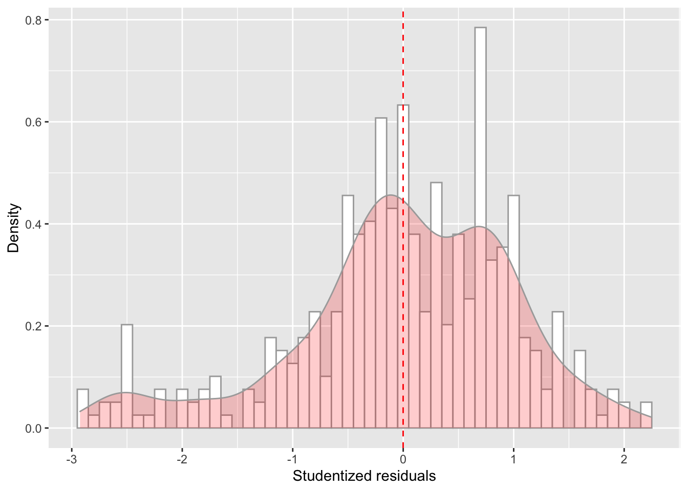
ggplot(model_checks, mapping = aes(sample = res_stu)) +
    stat_qq() +
    stat_qq_line()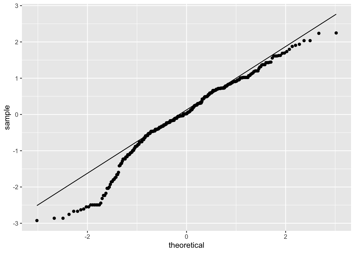
ggplot(data = model_checks, mapping = aes(x = pred, y = res_stu)) +
    geom_point(alpha = 0.6, size= 2) +
    geom_hline(yintercept=0)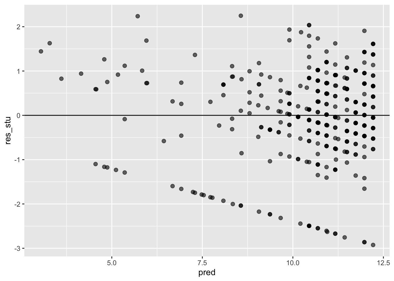
shapiro.test(model_checks$res_stu)##
## Shapiro-Wilk normality test
##
## data: model_checks$res_stu
## W = 0.96112, p-value = 1.007e-08bptest(model_fit_1)##
## studentized Breusch-Pagan test
##
## data: model_fit_1
## BP = 6.9372, df = 4, p-value = 0.1392# It looks like age and failure are actually correlated.
# This could affect interpretation of the corresponding coefficients.
# It also looks like the residuals are not normally distriburted.- Load the
student-por.csvin R asstudent_port. Inspect the dataset first.
student_por = read_csv2('data/student-por.csv')## ℹ Using "','" as decimal and "'.'" as grouping mark. Use `read_delim()` for more control.##
## ── Column specification ─────────────────────────────────────────────────────────────────────────────────────────────
## cols(
## .default = col_character(),
## age = col_double(),
## Medu = col_double(),
## Fedu = col_double(),
## traveltime = col_double(),
## studytime = col_double(),
## failures = col_double(),
## famrel = col_double(),
## freetime = col_double(),
## goout = col_double(),
## Dalc = col_double(),
## Walc = col_double(),
## health = col_double(),
## absences = col_double(),
## G1 = col_double(),
## G2 = col_double(),
## G3 = col_double()
## )
## ℹ Use `spec()` for the full column specifications.glimpse(student_por)## Rows: 649
## Columns: 33
## $ school <chr> "GP", "GP", "GP", "GP", "GP", "GP", "GP", "GP", "GP", "GP", "GP", "GP", "GP", "GP", "GP", "GP", …
## $ sex <chr> "F", "F", "F", "F", "F", "M", "M", "F", "M", "M", "F", "F", "M", "M", "M", "F", "F", "F", "M", "…
## $ age <dbl> 18, 17, 15, 15, 16, 16, 16, 17, 15, 15, 15, 15, 15, 15, 15, 16, 16, 16, 17, 16, 15, 15, 16, 16, …
## $ address <chr> "U", "U", "U", "U", "U", "U", "U", "U", "U", "U", "U", "U", "U", "U", "U", "U", "U", "U", "U", "…
## $ famsize <chr> "GT3", "GT3", "LE3", "GT3", "GT3", "LE3", "LE3", "GT3", "LE3", "GT3", "GT3", "GT3", "LE3", "GT3"…
## $ Pstatus <chr> "A", "T", "T", "T", "T", "T", "T", "A", "A", "T", "T", "T", "T", "T", "A", "T", "T", "T", "T", "…
## $ Medu <dbl> 4, 1, 1, 4, 3, 4, 2, 4, 3, 3, 4, 2, 4, 4, 2, 4, 4, 3, 3, 4, 4, 4, 4, 2, 2, 2, 2, 4, 3, 4, 4, 4, …
## $ Fedu <dbl> 4, 1, 1, 2, 3, 3, 2, 4, 2, 4, 4, 1, 4, 3, 2, 4, 4, 3, 2, 3, 3, 4, 2, 2, 4, 2, 2, 2, 4, 4, 4, 4, …
## $ Mjob <chr> "at_home", "at_home", "at_home", "health", "other", "services", "other", "other", "services", "o…
## $ Fjob <chr> "teacher", "other", "other", "services", "other", "other", "other", "teacher", "other", "other",…
## $ reason <chr> "course", "course", "other", "home", "home", "reputation", "home", "home", "home", "home", "repu…
## $ guardian <chr> "mother", "father", "mother", "mother", "father", "mother", "mother", "mother", "mother", "mothe…
## $ traveltime <dbl> 2, 1, 1, 1, 1, 1, 1, 2, 1, 1, 1, 3, 1, 2, 1, 1, 1, 3, 1, 1, 1, 1, 1, 2, 1, 1, 1, 1, 1, 1, 1, 2, …
## $ studytime <dbl> 2, 2, 2, 3, 2, 2, 2, 2, 2, 2, 2, 3, 1, 2, 3, 1, 3, 2, 1, 1, 2, 1, 2, 2, 3, 1, 1, 1, 2, 2, 2, 2, …
## $ failures <dbl> 0, 0, 0, 0, 0, 0, 0, 0, 0, 0, 0, 0, 0, 0, 0, 0, 0, 0, 3, 0, 0, 0, 0, 0, 0, 0, 0, 0, 0, 0, 0, 0, …
## $ schoolsup <chr> "yes", "no", "yes", "no", "no", "no", "no", "yes", "no", "no", "no", "no", "no", "no", "no", "no…
## $ famsup <chr> "no", "yes", "no", "yes", "yes", "yes", "no", "yes", "yes", "yes", "yes", "yes", "yes", "yes", "…
## $ paid <chr> "no", "no", "no", "no", "no", "no", "no", "no", "no", "no", "no", "no", "no", "no", "no", "no", …
## $ activities <chr> "no", "no", "no", "yes", "no", "yes", "no", "no", "no", "yes", "no", "yes", "yes", "no", "no", "…
## $ nursery <chr> "yes", "no", "yes", "yes", "yes", "yes", "yes", "yes", "yes", "yes", "yes", "yes", "yes", "yes",…
## $ higher <chr> "yes", "yes", "yes", "yes", "yes", "yes", "yes", "yes", "yes", "yes", "yes", "yes", "yes", "yes"…
## $ internet <chr> "no", "yes", "yes", "yes", "no", "yes", "yes", "no", "yes", "yes", "yes", "yes", "yes", "yes", "…
## $ romantic <chr> "no", "no", "no", "yes", "no", "no", "no", "no", "no", "no", "no", "no", "no", "no", "yes", "no"…
## $ famrel <dbl> 4, 5, 4, 3, 4, 5, 4, 4, 4, 5, 3, 5, 4, 5, 4, 4, 3, 5, 5, 3, 4, 5, 4, 5, 4, 1, 4, 2, 5, 4, 5, 4, …
## $ freetime <dbl> 3, 3, 3, 2, 3, 4, 4, 1, 2, 5, 3, 2, 3, 4, 5, 4, 2, 3, 5, 1, 4, 4, 5, 4, 3, 2, 2, 2, 3, 4, 4, 3, …
## $ goout <dbl> 4, 3, 2, 2, 2, 2, 4, 4, 2, 1, 3, 2, 3, 3, 2, 4, 3, 2, 5, 3, 1, 2, 1, 4, 2, 2, 2, 4, 3, 5, 2, 1, …
## $ Dalc <dbl> 1, 1, 2, 1, 1, 1, 1, 1, 1, 1, 1, 1, 1, 1, 1, 1, 1, 1, 2, 1, 1, 1, 1, 2, 1, 1, 1, 2, 1, 5, 3, 1, …
## $ Walc <dbl> 1, 1, 3, 1, 2, 2, 1, 1, 1, 1, 2, 1, 3, 2, 1, 2, 2, 1, 4, 3, 1, 1, 3, 4, 1, 3, 2, 4, 1, 5, 4, 1, …
## $ health <dbl> 3, 3, 3, 5, 5, 5, 3, 1, 1, 5, 2, 4, 5, 3, 3, 2, 2, 4, 5, 5, 1, 5, 5, 5, 5, 5, 5, 1, 5, 5, 5, 5, …
## $ absences <dbl> 4, 2, 6, 0, 0, 6, 0, 2, 0, 0, 2, 0, 0, 0, 0, 6, 10, 2, 2, 6, 0, 0, 0, 2, 2, 6, 8, 0, 2, 4, 0, 2,…
## $ G1 <dbl> 0, 9, 12, 14, 11, 12, 13, 10, 15, 12, 14, 10, 12, 12, 14, 17, 13, 13, 8, 12, 12, 11, 12, 10, 10,…
## $ G2 <dbl> 11, 11, 13, 14, 13, 12, 12, 13, 16, 12, 14, 12, 13, 12, 14, 17, 13, 14, 8, 12, 13, 12, 13, 10, 1…
## $ G3 <dbl> 11, 11, 12, 14, 13, 13, 13, 13, 17, 13, 14, 13, 12, 13, 15, 17, 14, 14, 7, 12, 14, 12, 14, 10, 1…- Create a new regression object called
model_fit_2using the same variables as question 1: however, this time use the portugese dataset.
model_fit_2 = lm(G3 ~ sex + age + internet + failures, data = student_por)
summary(model_fit_2)
##
## Call:
## lm(formula = G3 ~ sex + age + internet + failures, data = student_por)
##
## Residuals:
## Min 1Q Median 3Q Max
## -12.8941 -1.8345 0.0522 1.8807 7.8041
##
## Coefficients:
## Estimate Std. Error t value Pr(>|t|)
## (Intercept) 11.61020 1.68101 6.907 1.19e-11 ***
## sexM -0.71515 0.23625 -3.027 0.002568 **
## age 0.01986 0.10031 0.198 0.843134
## internetyes 0.92639 0.27508 3.368 0.000803 ***
## failures -2.04819 0.20738 -9.877 < 2e-16 ***
## ---
## Signif. codes: 0 '***' 0.001 '**' 0.01 '*' 0.05 '.' 0.1 ' ' 1
##
## Residual standard error: 2.936 on 644 degrees of freedom
## Multiple R-squared: 0.1794, Adjusted R-squared: 0.1743
## F-statistic: 35.19 on 4 and 644 DF, p-value: < 2.2e-16- What are the key differences between the beta values for the
portugese dataset (
model_fit_2) and the math dataset (model_fit_1)?
In the portugese datset, men do worse than women (b = -0.72, p < .01), and internet actually helps performance (b = 0.93, p < .01). Failures still lower grades (b = -2.05, p < .01).
Task B
- Using the
student_mathdataset, create a regression object calledmodel_fit_3predicting first period grade (G1) based on guardian. Guardian is a nominal variable with 3 levels.
model_fit_3 = lm(G1 ~ guardian, data = student_math)- Use
summaryto look at the output. You should see 2 predictors listed (“guardianmother” and “guardiananother”), rather than the expected 1 (“guardian”).lmhas dummy coded your variables with “father” set as the reference group. Look at the levels of the guardian factor to see why “father” is the reference group. How would you interpret the results?
summary(model_fit_3)##
## Call:
## lm(formula = G1 ~ guardian, data = student_math)
##
## Residuals:
## Min 1Q Median 3Q Max
## -7.8828 -2.8828 -0.1111 2.1172 8.1172
##
## Coefficients:
## Estimate Std. Error t value Pr(>|t|)
## (Intercept) 11.1111 0.3505 31.705 <2e-16 ***
## guardianmother -0.2283 0.4041 -0.565 0.572
## guardianother -0.5486 0.6843 -0.802 0.423
## ---
## Signif. codes: 0 '***' 0.001 '**' 0.01 '*' 0.05 '.' 0.1 ' ' 1
##
## Residual standard error: 3.325 on 392 degrees of freedom
## Multiple R-squared: 0.001775, Adjusted R-squared: -0.003318
## F-statistic: 0.3486 on 2 and 392 DF, p-value: 0.7059- What is the predicted grade for those with a father as their guardian? Those with a mother? Those with other? Compare these to the means of each group again.
We can use our three estimates to calculate these predictions. Father is a reference group/coded as 0, so the predicted grade is the intercept estimate (11.11). For the other two groups we just need to add their estimate to the intercept, therefore our predicted grade for those with a mother is 10.88 and for those with other it is 10.56.
summarize(group_by(student_math, guardian),
          mean_G1 = mean(G1))
## # A tibble: 3 x 2
## guardian mean_G1
## <chr> <dbl>
## 1 father 11.1
## 2 mother 10.9
## 3 other 10.6Task C
- Using the
student_mathdataset, create a regression object calledmodel_fit_4predicting a student’s first period grade (G1) based on all variables in the dataset (Hint: use the notationformula = y ~ .to include all variables)
model_fit_4 = lm(G1 ~ ., data = student_math)- Save the fitted values from the
model_fit_4object as a vector calledmodel_4_fitted.
model_4_fitted = model_fit_4$fitted.values

student_math$predicted_values = model_4_fitted- Using the
student_mathdataset, create a scatterplot showing the relationship between a student’s first period grade (G1) and the fitted values from the model. Does the model appear to correctly fit a student’s first period grade? Usegeom_abline()withslope=1andintercept=0to plot the identity line and better answer to this question.
ggplot(data = student_math, aes(x = G1, y = predicted_values)) +
  geom_jitter(alpha=.5, size=1) +
  geom_abline(slope=1, intercept=0, color='maroon', alpha=.5) +
  labs(x='Actual grade', y='Predicted grade')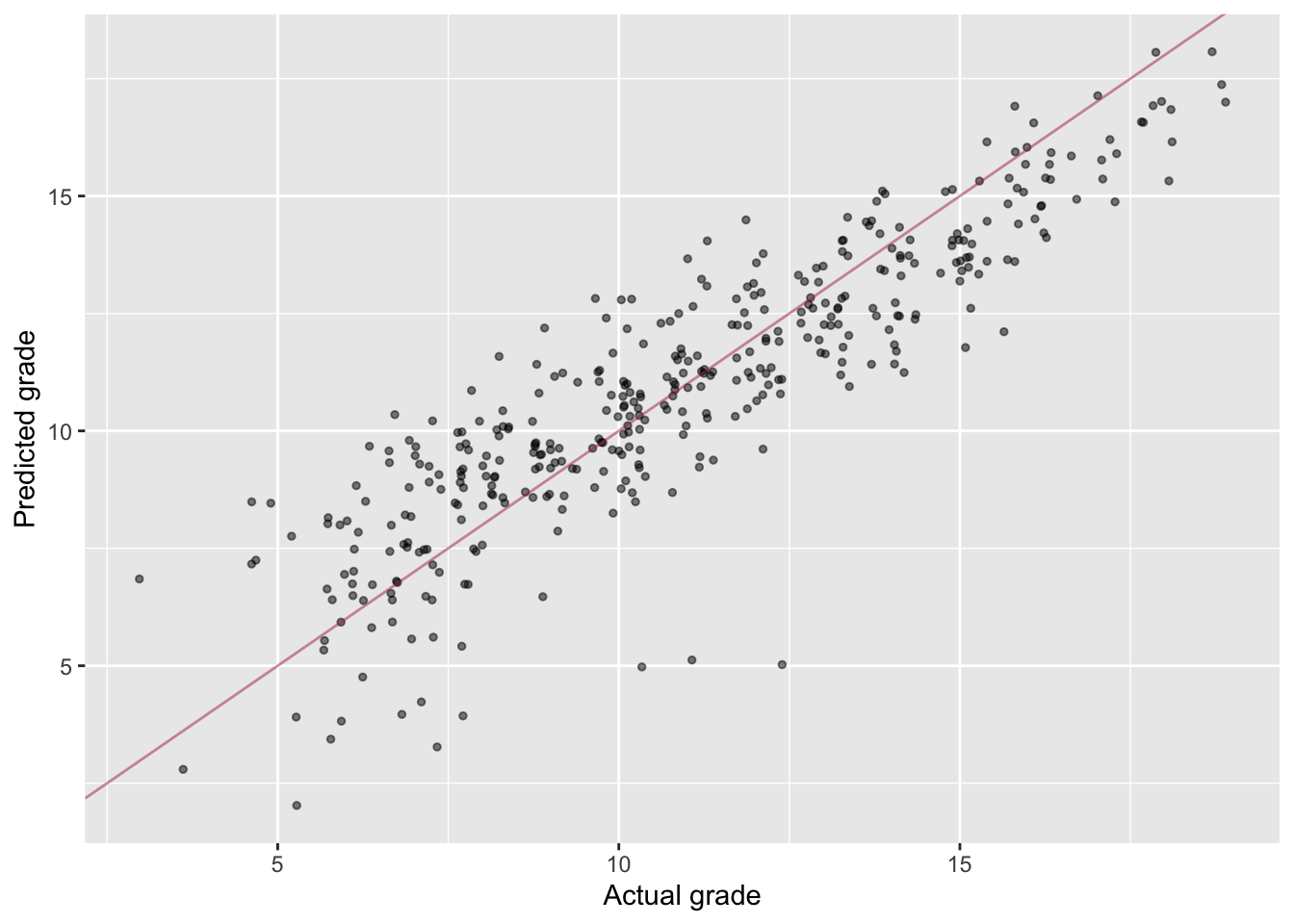
# Yes it seems to work well.
# This is probably because we are including both G2 and G3 as predictors.- Create a new regression object, called
model_fit_5which doesn’t include G2 or G3 as predictors, but still includes all other variables. Save the fitted values from themodel_fit_5object as a vector calledmodel_5_fitted.
model_fit_5 = lm(G1 ~ ., data = select(student_math, -predicted_values, -G2, -G3))

model_5_fitted = model_fit_5$fitted.values

student_math$predicted_values = model_5_fitted

summary(model_fit_5)
##
## Call:
## lm(formula = G1 ~ ., data = select(student_math, -predicted_values,
## -G2, -G3))
##
## Residuals:
## Min 1Q Median 3Q Max
## -6.5043 -1.9410 -0.0326 1.7997 7.1376
##
## Coefficients: (2 not defined because of singularities)
## Estimate Std. Error t value Pr(>|t|)
## (Intercept) 11.375064 3.113004 3.654 0.000297 ***
## schoolMS 0.009965 0.549925 0.018 0.985553
## sexM 0.894290 0.347385 2.574 0.010448 *
## age -0.070082 0.150905 -0.464 0.642639
## addressU 0.150710 0.405805 0.371 0.710571
## famsizeLE3 0.429175 0.339195 1.265 0.206602
## PstatusT 0.154297 0.502913 0.307 0.759170
## Medu 0.117943 0.224515 0.525 0.599688
## Fedu 0.143774 0.192870 0.745 0.456496
## Mjobhealth 0.926137 0.776837 1.192 0.233983
## Mjobother -0.782287 0.495455 -1.579 0.115244
## Mjobservices 0.466532 0.554282 0.842 0.400529
## Mjobteacher -0.922790 0.721274 -1.279 0.201596
## Fjobhealth -0.553377 0.998994 -0.554 0.579973
## Fjobother -1.134849 0.710736 -1.597 0.111217
## Fjobservices -0.994008 0.734310 -1.354 0.176705
## Fjobteacher 1.187017 0.900744 1.318 0.188414
## reasonhome 0.165602 0.384744 0.430 0.667150
## reasonother -0.181207 0.567991 -0.319 0.749891
## reasonreputation 0.444004 0.400557 1.108 0.268411
## guardianmother 0.050219 0.379042 0.132 0.894673
## guardianother 0.866380 0.694357 1.248 0.212947
## traveltime -0.025119 0.235489 -0.107 0.915112
## studytime 0.604725 0.199842 3.026 0.002659 **
## failures -1.314183 0.231280 -5.682 2.77e-08 ***
## schoolsupyes -2.155394 0.463335 -4.652 4.65e-06 ***
## famsupyes -0.978681 0.332560 -2.943 0.003466 **
## paidyes -0.102389 0.331906 -0.308 0.757892
## activitiesyes -0.052728 0.309114 -0.171 0.864652
## nurseryyes 0.029587 0.381623 0.078 0.938245
## higheryes 1.140610 0.748777 1.523 0.128575
## internetyes 0.255412 0.430423 0.593 0.553293
## romanticyes -0.211223 0.326001 -0.648 0.517455
## famrel 0.025733 0.170852 0.151 0.880363
## freetime 0.254817 0.164896 1.545 0.123161
## goout -0.413594 0.155971 -2.652 0.008367 **
## Dalc -0.063146 0.229869 -0.275 0.783703
## Walc -0.025339 0.172300 -0.147 0.883164
## health -0.167531 0.111859 -1.498 0.135102
## absences 0.012277 0.020124 0.610 0.542204
## sex_binary NA NA NA NA
## internet_binary NA NA NA NA
## ---
## Signif. codes: 0 '***' 0.001 '**' 0.01 '*' 0.05 '.' 0.1 ' ' 1
##
## Residual standard error: 2.854 on 355 degrees of freedom
## Multiple R-squared: 0.3339, Adjusted R-squared: 0.2607
## F-statistic: 4.562 on 39 and 355 DF, p-value: 3.633e-15- Plot the predicted grades against the actual ones, as predicted by
model
model_fit_5, as in question 3. How well does the new model perform now?
ggplot(data = student_math, aes(x = G1, y = predicted_values)) +
  geom_jitter(alpha=.5, size=1) +
  geom_abline(slope=1, intercept=0, color='maroon', alpha=.5) +
  labs(x='Actual grade', y='Predicted grade')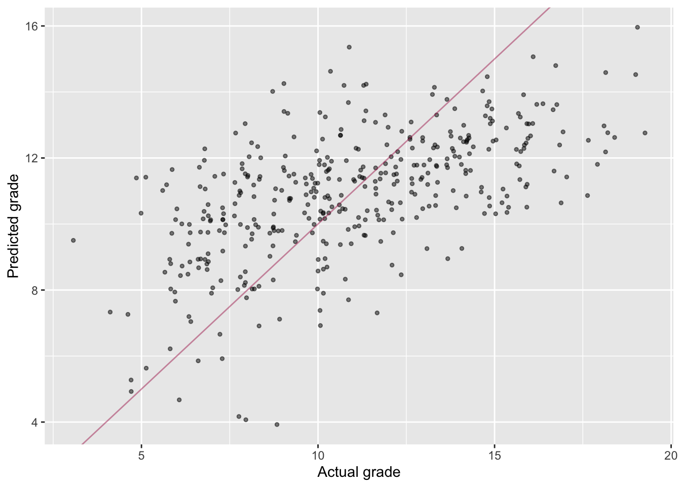
# It's performing a lot worse (Actually still explains like 30% of the variability so not that bad)Task D
For each question, conduct the appropriate ANOVA. Write the conclusion in APA style. To summarize an effect in an ANOVA, use the format F(XXX, YYY) = FFF, p = PPP, where XXX is the degrees of freedom of the variable you are testing, YYY is the degrees of freedom of the residuals, FFF is the F value for the variable you are testing, and PPP is the p-value. If the p-value is less than .01, just write p < .01.
For the purposes of this class, if the p-value of the ANOVA is less than .05, conduct post-hoc tests. If you are only testing one independent variable, write APA conclusions for the post-hoc test. If you are testing more than one independent variable in your ANOVA, you do not need to write APA style conclusions for post-hoc tests – just comment the result.
- Using the
student_mathdataset, was there a main effect of the school support on G1? Conduct a one-way ANOVA. If the result is significant (p < .05), conduct post-hoc tests.
aov_1 = aov(formula = G1 ~ schoolsup,
            data = student_math)

summary(aov_1)
## Df Sum Sq Mean Sq F value Pr(>F)
## schoolsup 1 196 196.21 18.61 2.04e-05 ***
## Residuals 393 4145 10.55
## ---
## Signif. codes: 0 '***' 0.001 '**' 0.01 '*' 0.05 '.' 0.1 ' ' 1TukeyHSD(aov_1)## Tukey multiple comparisons of means
## 95% family-wise confidence level
##
## Fit: aov(formula = G1 ~ schoolsup, data = student_math)
##
## $schoolsup
## diff lwr upr p adj
## yes-no -2.101801 -3.059794 -1.143808 2.04e-05There was a significant main effect of school support on the first period grade (F(1, 393) = 18.61, p < .01). Pairwise Tukey HSD tests showed significant differences between presence and absence of support (diff = -2.10, p < .01), with students with school support having on average a better grade.
- Using the
student_mathdataset, was there a main effect of the family support on G1? Conduct a one-way ANOVA. If the result is significant (p < .05), conduct post-hoc tests.
aov_2 = aov(formula = G1 ~ famsup,
            data = student_math)

summary(aov_2)
## Df Sum Sq Mean Sq F value Pr(>F)
## famsup 1 31 31.04 2.831 0.0933 .
## Residuals 393 4310 10.97
## ---
## Signif. codes: 0 '***' 0.001 '**' 0.01 '*' 0.05 '.' 0.1 ' ' 1There was no significant main effect of family support on the first period grade (F(1, 393) = 2.83, p = .09).
- Conduct a two-way ANOVA on G1 with both school support and family support as IVs. Do your results for each variable change compared to your previous one-way ANOVAs on these variables? (You do not need to give APA results or conduct post-hoc tests, just answer the question verbally).
aov_3 = aov(formula = G1 ~ schoolsup*famsup,
            data = student_math)

summary(aov_3)
## Df Sum Sq Mean Sq F value Pr(>F)
## schoolsup 1 196 196.21 18.595 2.05e-05 ***
## famsup 1 17 17.04 1.615 0.205
## schoolsup:famsup 1 2 1.69 0.160 0.689
## Residuals 391 4126 10.55
## ---
## Signif. codes: 0 '***' 0.001 '**' 0.01 '*' 0.05 '.' 0.1 ' ' 1No, we would come to the same conclusions.