final_project_solutions
Part 1
Part 1.1: Loading the data
library(tidyverse)

# define the data folder
data_folder = '~/Dropbox/teaching/r-course22/data/final_project/'

# define lists of files
list_files = paste(data_folder, list.files(path=data_folder), sep="")

# apply the read_delim function to each element in the list
data_list = lapply(list_files, function(x) read_delim(x, delim='\t'))

# loop through all the participants to add the participant number as a column as well as the name of the file, since we have no other way to know in which conditions the participants were in
data = NULL
participant = 0

for (n in 1:(length(data_list))){
    participant = participant + 1
    cond_list = strsplit(list_files[n], "_")
    condition = paste(cond_list[[1]][3], "_", cond_list[[1]][4], sep="")
    data=rbind(data,cbind(participant=participant, condition=condition, data_list[[n]]))
}head(data)## participant condition blkNum trlNum coherentDots numberofDots percentCoherence winningDirection response correct
## 1 1 Norm_Time 1 1 4 40 10 left left 1
## 2 1 Norm_Time 1 2 4 40 10 left right 0
## 3 1 Norm_Time 1 3 4 40 10 right left 0
## 4 1 Norm_Time 1 4 4 40 10 right left 0
## 5 1 Norm_Time 1 5 4 40 10 left left 1
## 6 1 Norm_Time 1 6 4 40 10 left left 1
## eventCount averageFrameRate RT
## 1 51 15.389 3314
## 2 40 15.250 2623
## 3 11 16.492 667
## 4 19 15.690 1211
## 5 99 15.175 6524
## 6 15 16.060 934As you can see, there are a few things to fix to make the dataset look a bit cleaner. It’s on you now to do the rest. The final data should consist of the following columns:
- participant
- block_number
- trial_number
- condition (use the labels in the description above)
- percent_coherence
- dots_direction
- response
- accuracy
- rt (change them to seconds, which means dividing them by 1000)
The columns in the dataset that are not in this list you should remove. The labels of the column that are different you should change to the ones below.
data = rename(data,
              block_number = blkNum,
              trial_number = trlNum,
              percent_coherence = percentCoherence,
              dots_direction = winningDirection,
              accuracy = correct,
              rt = RT)

data = mutate(data,
              condition = recode(condition,
                                 Norm_Trial = "FixedTrial_LowInformation",
                                 Info_Trial = "FixedTrial_MediumInformation",
                                 Optim_Trial = "FixedTrial_HighInformation",
                                 Norm_Time = "FixedTime_LowInformation",
                                 Info_Time = "FixedTime_MediumInformation",
                                 Optim_Time = "FixedTime_HighInformation"),
              rt = rt/1000)

data = select(data, -c("coherentDots", "numberofDots", "eventCount", "averageFrameRate"))

head(data)
## participant condition block_number trial_number percent_coherence dots_direction response accuracy
## 1 1 FixedTime_LowInformation 1 1 10 left left 1
## 2 1 FixedTime_LowInformation 1 2 10 left right 0
## 3 1 FixedTime_LowInformation 1 3 10 right left 0
## 4 1 FixedTime_LowInformation 1 4 10 right left 0
## 5 1 FixedTime_LowInformation 1 5 10 left left 1
## 6 1 FixedTime_LowInformation 1 6 10 left left 1
## rt
## 1 3.314
## 2 2.623
## 3 0.667
## 4 1.211
## 5 6.524
## 6 0.934Part 1.2: Describing the data
- How many participants are in the dataset?
summarize(data, n_distinct(participant))## n_distinct(participant)
## 1 85- How many participants were there in each condition?
summarize(group_by(data, condition), n_distinct(participant))## # A tibble: 6 x 2
## condition `n_distinct(participant)`
## <chr> <int>
## 1 FixedTime_HighInformation 14
## 2 FixedTime_LowInformation 16
## 3 FixedTime_MediumInformation 16
## 4 FixedTrial_HighInformation 13
## 5 FixedTrial_LowInformation 13
## 6 FixedTrial_MediumInformation 13- Did the participants in the fixed time conditions perform more or less trials than the participants in the fixed trials conditions?
data = mutate(data,
              blocktype = recode(condition,
                                 FixedTrial_LowInformation = "FixedTrial",
                                 FixedTrial_MediumInformation = "FixedTrial",
                                 FixedTrial_HighInformation = "FixedTrial",
                                 FixedTime_LowInformation = "FixedTime",
                                 FixedTime_MediumInformation = "FixedTime",
                                 FixedTime_HighInformation = "FixedTime"))

trials_blocktype = left_join(summarize(group_by(data, participant), n_trials=n()),
                             distinct(data, participant, blocktype),
                             by="participant")

summarize(group_by(trials_blocktype, blocktype), mean=mean(n_trials))
## # A tibble: 2 x 2
## blocktype mean
## <chr> <dbl>
## 1 FixedTime 775.
## 2 FixedTrial 960- Calculate a summary, which includes the average and SD of accuracy and response time per condition (which are 6 in total) and use this to describe the overall performance across participants in these conditions (i.e., which conditions produced hiigher accuracy, which produced faster responses? Do accuracy and speed always trade off?).
summarize(group_by(data, condition), meanRT=mean(rt), meanACC=mean(accuracy))## # A tibble: 6 x 3
## condition meanRT meanACC
## <chr> <dbl> <dbl>
## 1 FixedTime_HighInformation 1.21 0.768
## 2 FixedTime_LowInformation 1.59 0.738
## 3 FixedTime_MediumInformation 1.33 0.801
## 4 FixedTrial_HighInformation 1.31 0.789
## 5 FixedTrial_LowInformation 1.16 0.794
## 6 FixedTrial_MediumInformation 1.12 0.785- Calculate a summary, which includes the average accuracy and average response time per participant, as well as the percentage of trials below 150 ms (too fast trials) and above 5000 ms (too slow trials). Are there any participants with more then 10% fast or slow trials?
data = mutate(data,
              slow_trials = case_when(
                rt >= 5 ~ 1,
                rt < 5 ~ 0),
              fast_trials = case_when(
                rt <= .15 ~ 1,
                rt > .15 ~ 0))

participant_performance = summarize(group_by(data, participant),
                                    meanRT=mean(rt),
                                    meanACC=mean(accuracy),
                                    perc_slow_trials = mean(slow_trials)*100,
                                    perc_fast_trials = mean(fast_trials)*100)
filter(participant_performance, perc_slow_trials >= 10)
## # A tibble: 7 x 5
## participant meanRT meanACC perc_slow_trials perc_fast_trials
## <dbl> <dbl> <dbl> <dbl> <dbl>
## 1 28 2.67 0.805 10.1 0
## 2 47 4.79 0.729 36.3 0
## 3 58 2.56 0.644 11.1 0.208
## 4 70 2.81 0.673 10.6 0
## 5 82 3.25 0.556 17.9 0
## 6 83 2.75 0.906 15.2 0
## 7 85 2.18 0.709 11.8 0filter(participant_performance, perc_fast_trials >= 10)## # A tibble: 0 x 5
## # … with 5 variables: participant <dbl>, meanRT <dbl>, meanACC <dbl>, perc_slow_trials <dbl>, perc_fast_trials <dbl>Part 1.3: Exclude participants
Exclude from the dataset the participants that have less than 60% accuracy. The trials with a response time less than 150 ms or greater than 5000 ms should be also excluded. Check that the accuracy variable only contains 0 and 1.
participants_to_exclude = filter(participant_performance, meanACC < .6)$participant

for (n in 1:length(participants_to_exclude)) {
  data = data %>%
    filter(participant != participants_to_exclude[n])
}
Part 1.4: Data visualization
Now it’s time to visualize the data set.
- First, we want to have a look at how the accuracy and response time evolve across the blocks. For this purpose, you should make a 2-by-1 grid plot that depicts the response time (top panel) and accuracy (lower panel) across the blocks for each condition. This should recreate Figure 2 fromt he paper: https://link.springer.com/article/10.3758/s13423-016-1135-1/figures/2 (excluding the top panel). What trends do you observe?
grouped_data = group_by(data, condition, block_number)
data_summary = summarise(grouped_data, meanRT = mean(rt), meanACC = mean(accuracy))
## `summarise()` has grouped output by 'condition'. You can override using the `.groups` argument.ggplot(data = data_summary, mapping = aes(x = block_number, y = meanACC, color=condition)) +
geom_line()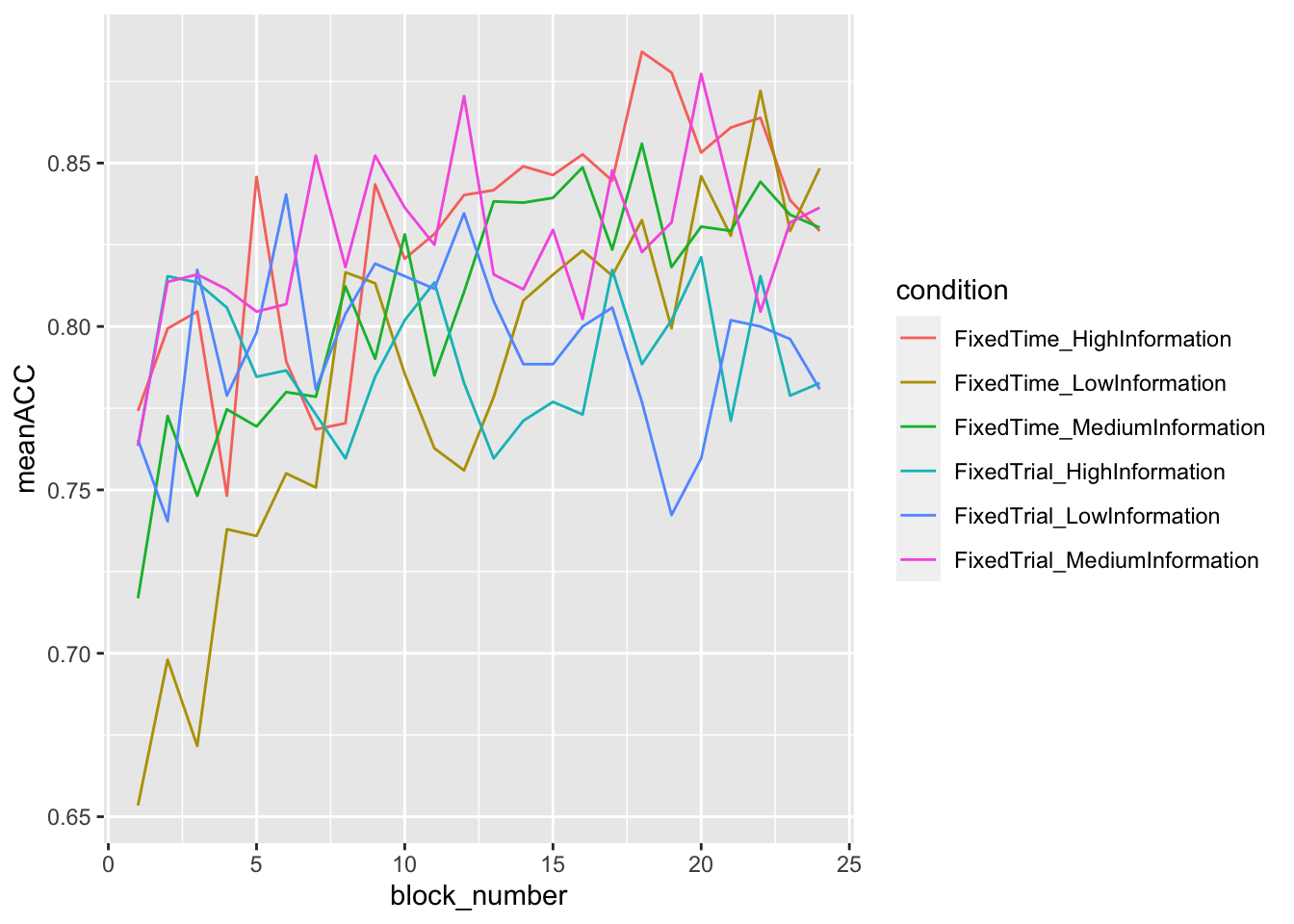
ggplot(data = data_summary, mapping = aes(x = block_number, y = meanRT, color=condition)) +
    geom_line()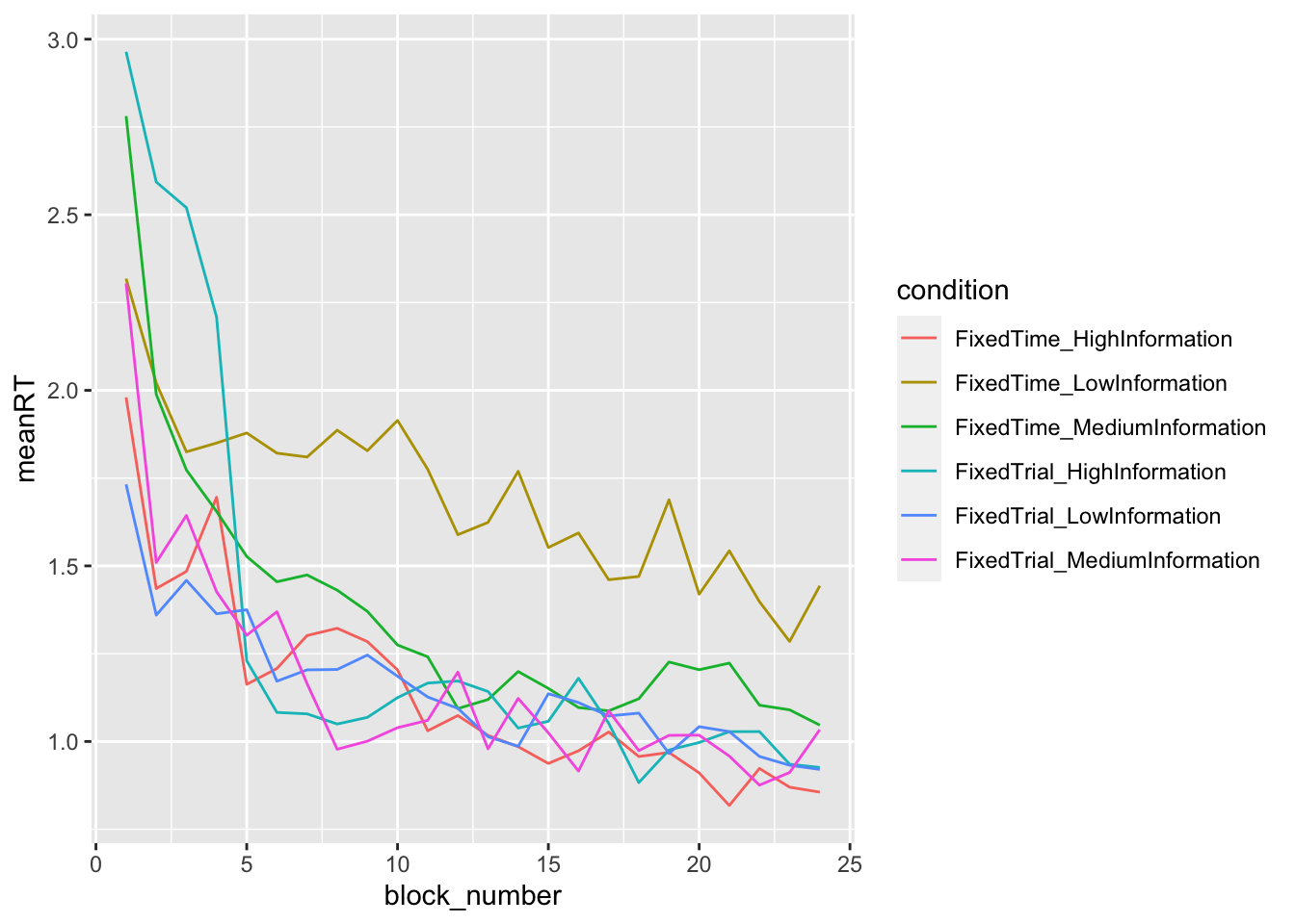
- Second, we want to make two separate plots, one for accuracy and one for response times, which show the average performance iin the 6 conditions. The condition should be plotted in the x-axis and the performance (either accuracy or rt) in the y-axis. You can choose whether you would like to have bar plots or point plots. Add error bars representing confidence intervals.
ggplot(data = data, mapping = aes(x = condition, y = accuracy)) +
    stat_summary(fun = "mean", geom="point", size=3) +
    stat_summary(fun.data = mean_cl_normal, geom = "errorbar", size=1, width=.2) +
    theme(axis.text.x = element_text(angle = 90))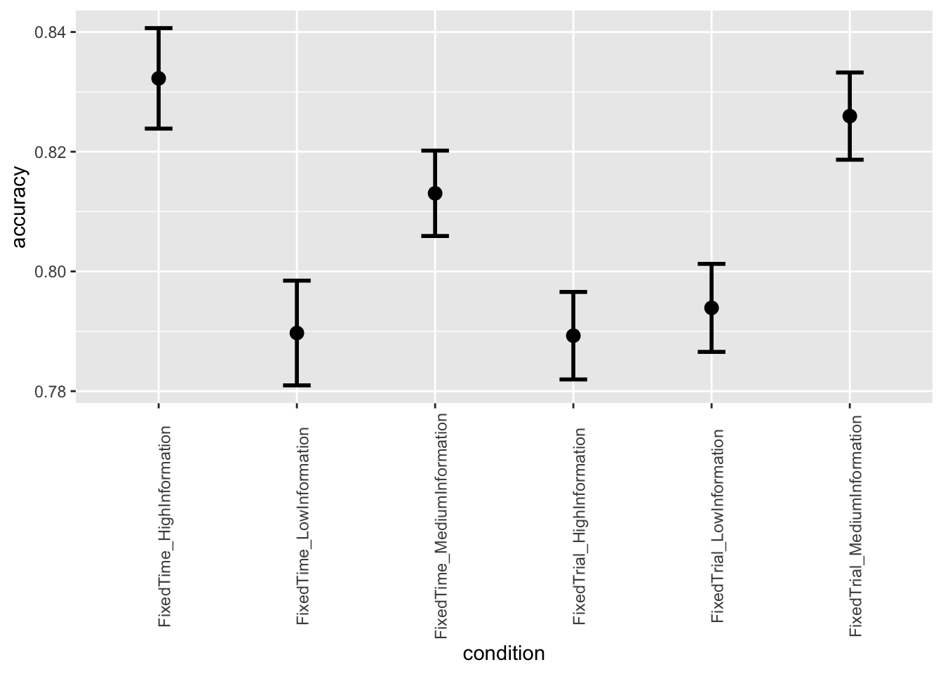
ggplot(data = data, mapping = aes(x = condition, y = rt)) +
    stat_summary(fun = "mean", geom="point", size=3) +
    stat_summary(fun.data = mean_cl_normal, geom = "errorbar", size=1, width=.2) +
    theme(axis.text.x = element_text(angle = 90))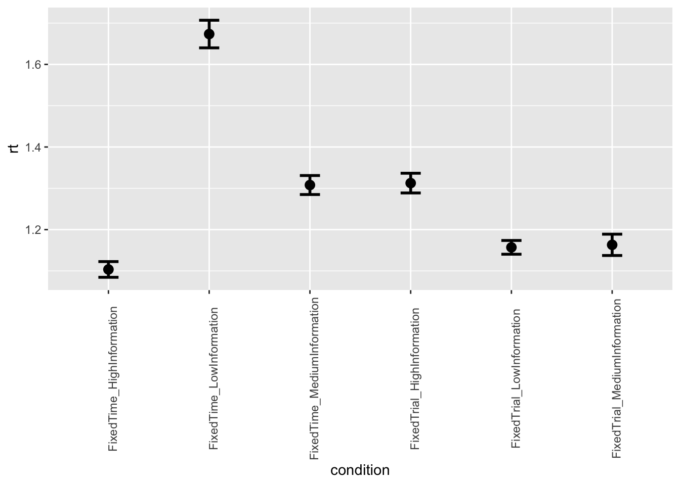
Alternatively:
data = mutate(data,
              trialtype = recode(condition,
                                 FixedTrial_LowInformation = "LowInformation",
                                 FixedTrial_MediumInformation = "MediumInformation",
                                 FixedTrial_HighInformation = "HighInformation",
                                 FixedTime_LowInformation = "LowInformation",
                                 FixedTime_MediumInformation = "MediumInformation",
                                 FixedTime_HighInformation = "HighInformation"))

ggplot(data = data, mapping = aes(x = trialtype, y = accuracy, color=blocktype)) +
    stat_summary(fun = "mean", geom="point", size=3) +
    stat_summary(fun.data = mean_cl_normal, geom = "errorbar", size=1, width=.2) +
    theme(axis.text.x = element_text(angle = 90))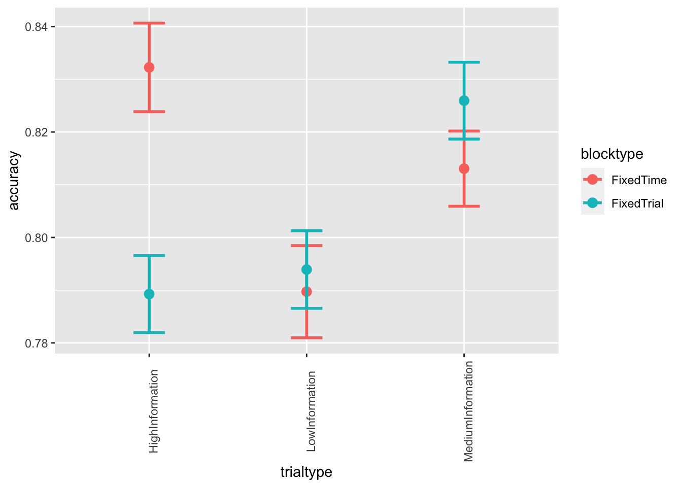
ggplot(data = data, mapping = aes(x = trialtype, y = rt, color=blocktype)) +
    stat_summary(fun = "mean", geom="point", size=3) +
    stat_summary(fun.data = mean_cl_normal, geom = "errorbar", size=1, width=.2) +
    theme(axis.text.x = element_text(angle = 90))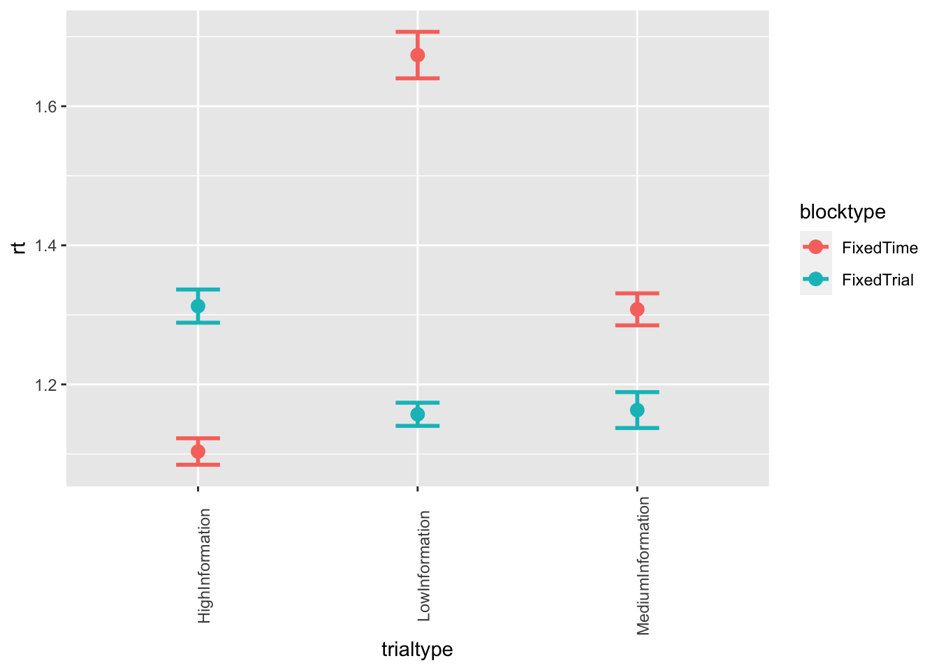
Part 1.5 Calculate the reward rate (option to do this for next week together with part 2)
In the paper, they define the reward rate as:
\(\frac {PC}{MRT + ITI + FDT + (1-PC)*ET}\)
where MRT and PC refer to the mean correct response time and probability of a correct response, ITI is the inter-trial interval (i.e., 100 ms), FDT is the feedback display time (i.e., 300 ms), and ET is the error timeout (i.e., 500 ms).
By calculating the MRT and PC per block per participant (i.e., create
a summary using participant and block_number
as grouping variables), you can calculate the reward_rate
by filling in the rest of the equation above.
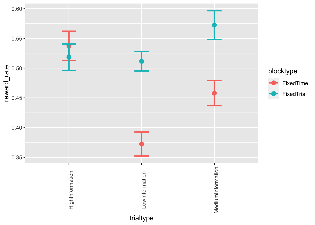
When you are done, you can add the reward rate to the plot in Part 1.4 (so recreate the full Figure 2 from the paper), and also plot the mean reward rate per condition, as you did in Part 1.4 for accuracy and RT.
grouped_data_pos = group_by(filter(data, accuracy > 0), participant, block_number)
grouped_data = group_by(data, participant, block_number)

data_summary = full_join(summarise(grouped_data_pos, MRT = mean(rt)),
                         summarise(grouped_data, PC = mean(accuracy)))
## `summarise()` has grouped output by 'participant'. You can override using the `.groups` argument.
## `summarise()` has grouped output by 'participant'. You can override using the `.groups` argument.## Joining, by = c("participant", "block_number")data_summary = full_join(data_summary,
distinct(data, participant, block_number, condition, blocktype, trialtype))## Joining, by = c("participant", "block_number")data_summary = mutate(data_summary,
reward_rate = PC/(MRT + .1 + .3 + (1 - PC)*.5))grouped_data_summary = group_by(data_summary, condition, block_number)
data_summary_summary = summarise(grouped_data_summary, meanRR = mean(reward_rate))## `summarise()` has grouped output by 'condition'. You can override using the `.groups` argument.ggplot(data = data_summary_summary, mapping = aes(x = block_number, y = meanRR, color=condition)) +
geom_line()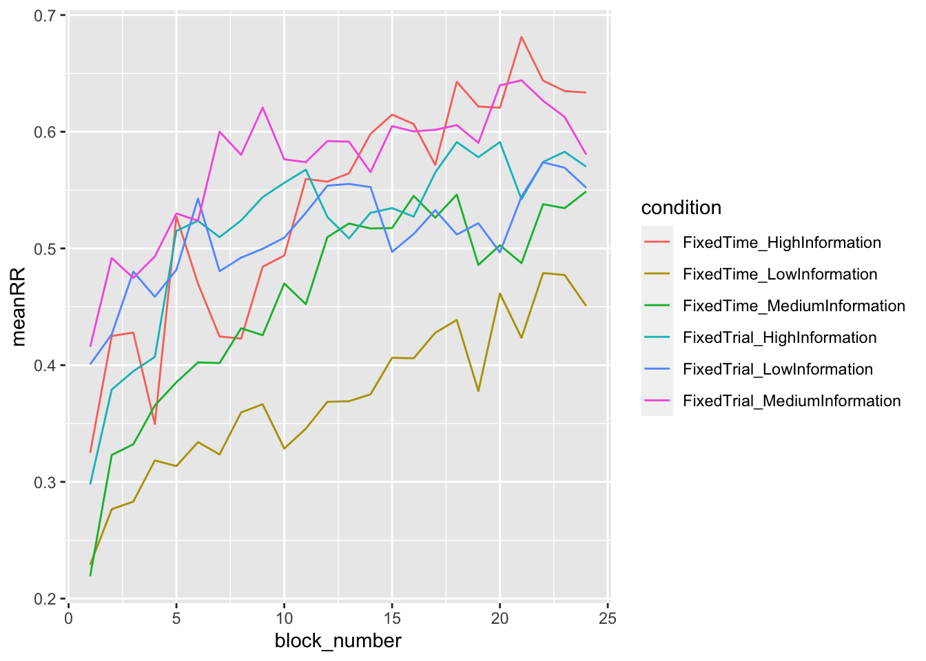
ggplot(data = data_summary, mapping = aes(x = trialtype, y = reward_rate, color=blocktype)) +
    stat_summary(fun = "mean", geom="point", size=3) +
    stat_summary(fun.data = mean_cl_normal, geom = "errorbar", size=1, width=.2) +
    theme(axis.text.x = element_text(angle = 90))