Introduction to Rstudio, and seeing what R can do
1. RStudio
Open RStudio.
RStudio panes
The RStudio interface consists of four main panes, or windows.
- Bottom left: console or command window. Here you can type any valid R command after the > prompt followed by Enter and R will execute that command.
- Top left: text editor or script window. This is where you can save and edit collections of commands.
- Top right: environment & history window. The environment window contains objects (data, values, functions) R has currently stored in its memory. The history window shows all commands that were executed in the console.
- Bottom right: files, plots, packages, help, & viewer pane. Here you can open files, view plots, install and load packages, read man pages, and view markdown and other documents in the viewer tab.
The location of these windows can be changed by clicking Tools > Global Options > Pane Layout.
You may have noticed that, by default, there is no text editor window open. In order to open one, click File > New File > R Script. Alternatively, click the ‘Add new document’ symbol and select R Script.
Open a new R script in R and save it as
wpa_1_LastFirst.R (where Last and First is your last and
first name).
Careful about capitalizing, and using _ and
not, e.g., WPA-1-LastFirst.R
At the top of your script, write the following (with appropriate changes):
# Assignment: WPA 1
# Name: Laura Fontanesi
# Date: 15 March 2022
Code completion
RStudio supports automatic completion of code using the Tab key.
For example, let’s create a new object, named
my_block_rewards:
my_block_rewards = c(34, 36, 90)Now, you can type my and then press Tab and RStudio will
automatically complete the full name of the object if my is
unique; otherwise, RStudio will list all of the objects (or functions)
starting with my in your current environment.
Try now to define another object starting with my and
see what happens.
my_score = .4Code completion also works for function arguments.
data() is a function to load one of R preset
dataframes.
Type data(m in the console, then hit Tab to bring up a
list of options. RStudio will automatically add a closing parenthesis
for you, but your cursor needs to be between the two parentheses for tab
completion to work.
Choose mtcars from the list and press Enter. What
happens?
Environment browser
The mtcars object should have appeared in your
environment tab.
The environment tab is in the top right window, which displays the R objects that exist in the global environment. These are the objects that were created by you in your current session.
If you click the load symbol next to the mtcars object,
you can see the structure of the object. You can also click the view
icon load to have a table view of the dataset. This might come useful at
times.
Run some code in your script file
What we want to do most of time is to run our code from the script and not from the console. This will help us writing more complicated functions and keep track of exactly what we have been doing up to that point.
You always have the choice to run part of it or the whole code. I suggest (particularly at the begginning) to always run from the start to the end of your code, and to make sure that your workspace is clean at the beginning.
It’s very useful to use shortcuts for this, for example:
| Description | Windows & Linux | Mac |
|---|---|---|
| Run current line/selection | Ctrl+Enter | Command+Enter |
| Run current line/selection (retain cursor position) | Alt+Enter | Option+Enter |
| Run current document | Ctrl+Alt+R | Command+Option+R |
| Run from document beginning to current line | Ctrl+Alt+B | Command+Option+B |
| Run from current line to document end | Ctrl+Alt+E | Command+Option+E |
See here for more.
Practice with the following chunk of code:
data(mtcars)

head(mtcars)
## mpg cyl disp hp drat wt qsec vs am gear carb
## Mazda RX4 21.0 6 160 110 3.90 2.620 16.46 0 1 4 4
## Mazda RX4 Wag 21.0 6 160 110 3.90 2.875 17.02 0 1 4 4
## Datsun 710 22.8 4 108 93 3.85 2.320 18.61 1 1 4 1
## Hornet 4 Drive 21.4 6 258 110 3.08 3.215 19.44 1 0 3 1
## Hornet Sportabout 18.7 8 360 175 3.15 3.440 17.02 0 0 3 2
## Valiant 18.1 6 225 105 2.76 3.460 20.22 1 0 3 1colnames(mtcars)## [1] "mpg" "cyl" "disp" "hp" "drat" "wt" "qsec" "vs" "am" "gear" "carb"colnames(mtcars)[1] = 'MPG'
head(mtcars)## MPG cyl disp hp drat wt qsec vs am gear carb
## Mazda RX4 21.0 6 160 110 3.90 2.620 16.46 0 1 4 4
## Mazda RX4 Wag 21.0 6 160 110 3.90 2.875 17.02 0 1 4 4
## Datsun 710 22.8 4 108 93 3.85 2.320 18.61 1 1 4 1
## Hornet 4 Drive 21.4 6 258 110 3.08 3.215 19.44 1 0 3 1
## Hornet Sportabout 18.7 8 360 175 3.15 3.440 17.02 0 0 3 2
## Valiant 18.1 6 225 105 2.76 3.460 20.22 1 0 3 1Retrieving previous commands
It’s often the case that you want to re-execute commands that you previously entered. The RStudio console supports the ability to recall previous commands using the arrow keys:
- Up — Recall previous command(s)
- Down — Reverse of Up
You can even view a list of your recent commands by pressing Ctrl+Up on Windows or Command+Up on a Mac.
See here for more RStudio tips.
2. Install and load packages
install.packages('tidyverse')library(tidyverse)3. Load and inspect some data
# load data without downloading

con = url('https://github.com/laurafontanesi/r-seminar22/blob/main/data/movies.RData?raw=true')
load(con)
close(con)
# command to list all the variables in your workspace
ls()## [1] "anova_fit" "con" "movies" "mtcars" "my_block_rewards" "my_score"
## [7] "regression_fit" "x"# inspect the first 5 lines of a dataset
movies %>%
slice(1:5)## # A tibble: 5 x 32
## title title_type genre runtime mpaa_rating studio thtr_rel_year thtr_rel_month thtr_rel_day dvd_rel_year
## <chr> <fct> <fct> <dbl> <fct> <fct> <dbl> <dbl> <dbl> <dbl>
## 1 Filly Brown Feature Film Drama 80 R Indom… 2013 4 19 2013
## 2 The Dish Feature Film Drama 101 PG-13 Warne… 2001 3 14 2001
## 3 Waiting for Guffman Feature Film Comedy 84 R Sony … 1996 8 21 2001
## 4 The Age of Innocence Feature Film Drama 139 PG Colum… 1993 10 1 2001
## 5 Malevolence Feature Film Horror 90 R Ancho… 2004 9 10 2005
## # … with 22 more variables: dvd_rel_month <dbl>, dvd_rel_day <dbl>, imdb_rating <dbl>, imdb_num_votes <int>,
## # critics_rating <fct>, critics_score <dbl>, audience_rating <fct>, audience_score <dbl>, best_pic_nom <fct>,
## # best_pic_win <fct>, best_actor_win <fct>, best_actress_win <fct>, best_dir_win <fct>, top200_box <fct>,
## # director <chr>, actor1 <chr>, actor2 <chr>, actor3 <chr>, actor4 <chr>, actor5 <chr>, imdb_url <chr>,
## # rt_url <chr>summary(movies)## title title_type genre runtime mpaa_rating
## Length:651 Documentary : 55 Drama :305 Min. : 39.0 G : 19
## Class :character Feature Film:591 Comedy : 87 1st Qu.: 92.0 NC-17 : 2
## Mode :character TV Movie : 5 Action & Adventure: 65 Median :103.0 PG :118
## Mystery & Suspense: 59 Mean :105.8 PG-13 :133
## Documentary : 52 3rd Qu.:115.8 R :329
## Horror : 23 Max. :267.0 Unrated: 50
## (Other) : 60 NA's :1
## studio thtr_rel_year thtr_rel_month thtr_rel_day dvd_rel_year
## Paramount Pictures : 37 Min. :1970 Min. : 1.00 Min. : 1.00 Min. :1991
## Warner Bros. Pictures : 30 1st Qu.:1990 1st Qu.: 4.00 1st Qu.: 7.00 1st Qu.:2001
## Sony Pictures Home Entertainment: 27 Median :2000 Median : 7.00 Median :15.00 Median :2004
## Universal Pictures : 23 Mean :1998 Mean : 6.74 Mean :14.42 Mean :2004
## Warner Home Video : 19 3rd Qu.:2007 3rd Qu.:10.00 3rd Qu.:21.00 3rd Qu.:2008
## (Other) :507 Max. :2014 Max. :12.00 Max. :31.00 Max. :2015
## NA's : 8 NA's :8
## dvd_rel_month dvd_rel_day imdb_rating imdb_num_votes critics_rating critics_score
## Min. : 1.000 Min. : 1.00 Min. :1.900 Min. : 180 Certified Fresh:135 Min. : 1.00
## 1st Qu.: 3.000 1st Qu.: 7.00 1st Qu.:5.900 1st Qu.: 4546 Fresh :209 1st Qu.: 33.00
## Median : 6.000 Median :15.00 Median :6.600 Median : 15116 Rotten :307 Median : 61.00
## Mean : 6.333 Mean :15.01 Mean :6.493 Mean : 57533 Mean : 57.69
## 3rd Qu.: 9.000 3rd Qu.:23.00 3rd Qu.:7.300 3rd Qu.: 58300 3rd Qu.: 83.00
## Max. :12.000 Max. :31.00 Max. :9.000 Max. :893008 Max. :100.00
## NA's :8 NA's :8
## audience_rating audience_score best_pic_nom best_pic_win best_actor_win best_actress_win best_dir_win top200_box
## Spilled:275 Min. :11.00 no :629 no :644 no :558 no :579 no :608 no :636
## Upright:376 1st Qu.:46.00 yes: 22 yes: 7 yes: 93 yes: 72 yes: 43 yes: 15
## Median :65.00
## Mean :62.36
## 3rd Qu.:80.00
## Max. :97.00
##
## director actor1 actor2 actor3 actor4 actor5
## Length:651 Length:651 Length:651 Length:651 Length:651 Length:651
## Class :character Class :character Class :character Class :character Class :character Class :character
## Mode :character Mode :character Mode :character Mode :character Mode :character Mode :character
##
##
##
##
## imdb_url rt_url
## Length:651 Length:651
## Class :character Class :character
## Mode :character Mode :character
##
##
##
## Continuous variables
# plot relationship between two variables, critics_score and audience_score

ggplot(data = movies, aes(x = critics_score, y = audience_score, color=imdb_rating)) +
  geom_jitter() +
  scale_colour_gradient(low = "blue", high = "gold", limits=range(movies[,'imdb_rating'])) +
  labs(x = "Critics Score", y = "Audience Score", color='IMDb rating') +
  ggtitle("Relationship Between Critics Score And Audience Score On Rotten Tomatoes")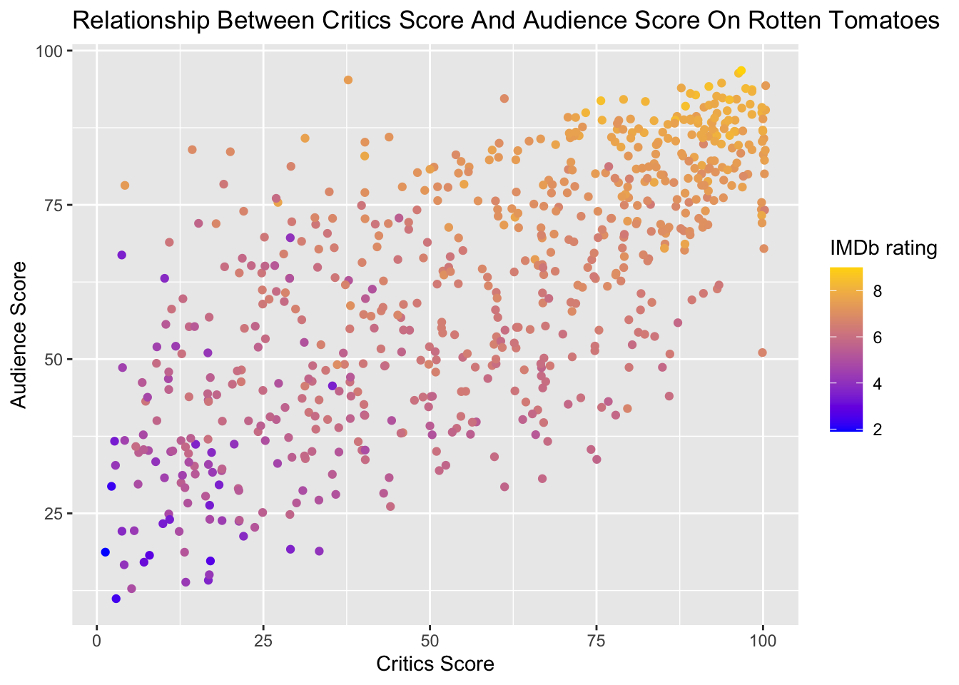
# Run a correlation test
cor.test(~ audience_score + critics_score, data = movies)
##
## Pearson's product-moment correlation
##
## data: audience_score and critics_score
## t = 25.273, df = 649, p-value < 2.2e-16
## alternative hypothesis: true correlation is not equal to 0
## 95 percent confidence interval:
## 0.6633319 0.7410163
## sample estimates:
## cor
## 0.7042762# Run a regression
regression_fit = lm(formula = audience_score ~ critics_score + imdb_rating,
data = movies)
# Print summary results
summary(regression_fit)##
## Call:
## lm(formula = audience_score ~ critics_score + imdb_rating, data = movies)
##
## Residuals:
## Min 1Q Median 3Q Max
## -26.668 -6.758 0.723 5.513 52.438
##
## Coefficients:
## Estimate Std. Error t value Pr(>|t|)
## (Intercept) -37.03195 2.86401 -12.930 < 2e-16 ***
## critics_score 0.07318 0.02161 3.386 0.000753 ***
## imdb_rating 14.65760 0.56590 25.901 < 2e-16 ***
## ---
## Signif. codes: 0 '***' 0.001 '**' 0.01 '*' 0.05 '.' 0.1 ' ' 1
##
## Residual standard error: 10.08 on 648 degrees of freedom
## Multiple R-squared: 0.7524, Adjusted R-squared: 0.7516
## F-statistic: 984.4 on 2 and 648 DF, p-value: < 2.2e-16cormat = cor(movies[, c('audience_score', 'critics_score', 'imdb_rating', 'imdb_num_votes')])
cormat## audience_score critics_score imdb_rating imdb_num_votes
## audience_score 1.0000000 0.7042762 0.8648652 0.2898128
## critics_score 0.7042762 1.0000000 0.7650355 0.2092508
## imdb_rating 0.8648652 0.7650355 1.0000000 0.3311525
## imdb_num_votes 0.2898128 0.2092508 0.3311525 1.0000000Discrete variables
ggplot(data = movies, aes(x = best_pic_nom, y = audience_score, fill = best_dir_win)) +
  geom_boxplot() +
  labs(x = "Movie Was Nominated For A Best Picture Oscar", y = "Audience Score", fill = "Director won oscar") +
  ggtitle("Relationship Between Audience Score, Movie Picture Oscar and Director Achievement")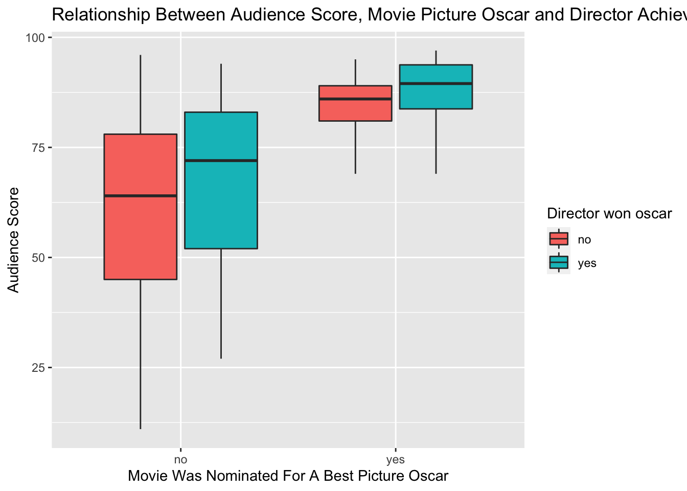
# Run an ANOVA
anova_fit = aov(formula = audience_score ~ best_pic_nom * best_dir_win,
                data = movies)

# Print summary results
summary(anova_fit)
## Df Sum Sq Mean Sq F value Pr(>F)
## best_pic_nom 1 11999 11999 30.712 4.36e-08 ***
## best_dir_win 1 1014 1014 2.597 0.108
## best_pic_nom:best_dir_win 1 38 38 0.097 0.756
## Residuals 647 252769 391
## ---
## Signif. codes: 0 '***' 0.001 '**' 0.01 '*' 0.05 '.' 0.1 ' ' 1ggplot(data = movies, aes(x = thtr_rel_year)) +
geom_bar() +
ggtitle("Number of movies in the database per release year") +
labs(x = "Theatrical release year", y = "Count")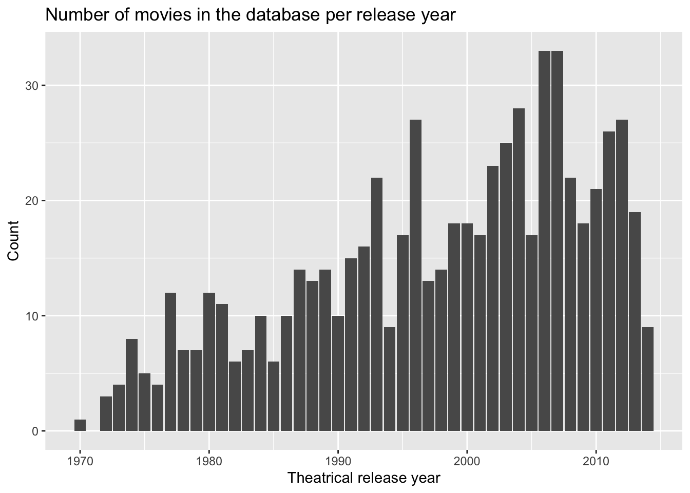
4. Now it’s your turn
Task A
- Plot the relationship between:
imdb_rating,imdb_num_votesandaudience_score. - Change the coloring of the scatterplot. You can either have a look here or simply change the two colors in the gradients, and have a look for example here.
- Compute the regression for such relationship.
Task B
- Plot the relationship between
best_actor_win,best_actress_winandaudience_score. - Compute the ANOVA for such relationship.
Task C
- Plot the number of movies in each
mpaa_ratingcategory.
Submit your assignment
Save and email your wpa_1_LastFirst.R script to me at laura.fontanesi@unibas.ch by
the end of the day.