Multiple regression and ANOVA

1. Multiple linear regression model

Last week we looked at linear models with 1 predictor (either continuous or categorical with 2 levels). Now we are going to extend this to linear models with more than 1 predictor.

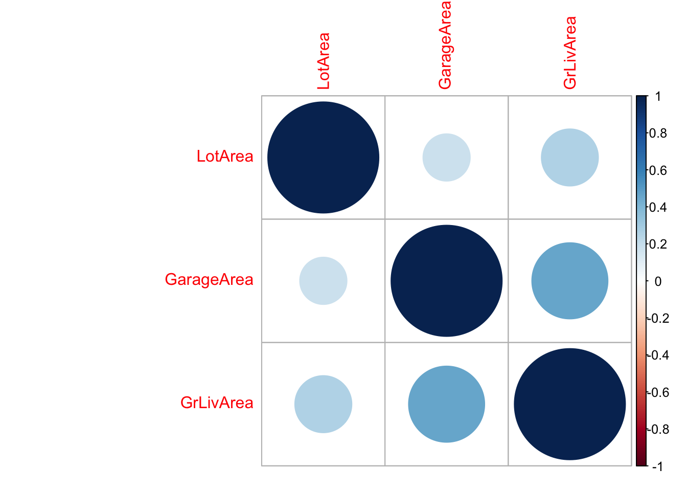
We have already seen the assumptions of multiple linear regression last week. They are essentially the same as for simple linear regression but now we should also check that the predictors are not correlated.

Open RStudio.

Open a new R script in R and save it as wpa_9_LastFirst.R (where Last and First is your last and first name).

Careful about: capitalizing, last and first name order, and using _ instead of -.

At the top of your script, write the following (with appropriate changes):

# Assignment: WPA 9
# Name: Laura Fontanesi
# Date: 9 May 2022

Model fitting

Model fit can be achieved as in simple linear regression using lm().

the only thing to take into account is how to change the formula argument:

• outcome ~ predictor1 + predictor2: tests main effects only of these two predictors
• outcome ~ predictor1 * predictor2: tests all main effects and the interaction effect of these two predictors
• outcome ~ predictor1 * predictor2 * predictor3: tests all main effects and all interaction effect of these three predictors
• outcome ~ predictor1 + predictor2 + predictor3 + predictor1*predictor2: tests main all three main effects and only the interaction effect of the first and second predictor

Download the house_prices.csv dataset from the Github folder and load it in R:

library(tidyverse)

house_prices = read_csv('data/house_prices.csv')

## 
## ── Column specification ─────────────────────────────────────────────────────────────────────────────────────────────
## cols(
##   .default = col_character(),
##   Id = col_double(),
##   MSSubClass = col_double(),
##   LotFrontage = col_double(),
##   LotArea = col_double(),
##   OverallQual = col_double(),
##   OverallCond = col_double(),
##   YearBuilt = col_double(),
##   YearRemodAdd = col_double(),
##   MasVnrArea = col_double(),
##   BsmtFinSF1 = col_double(),
##   BsmtFinSF2 = col_double(),
##   BsmtUnfSF = col_double(),
##   TotalBsmtSF = col_double(),
##   `1stFlrSF` = col_double(),
##   `2ndFlrSF` = col_double(),
##   LowQualFinSF = col_double(),
##   GrLivArea = col_double(),
##   BsmtFullBath = col_double(),
##   BsmtHalfBath = col_double(),
##   FullBath = col_double()
##   # ... with 18 more columns
## )
## ℹ Use `spec()` for the full column specifications.

glimpse(house_prices)

## Rows: 1,460
## Columns: 81
## $ Id            <dbl> 1, 2, 3, 4, 5, 6, 7, 8, 9, 10, 11, 12, 13, 14, 15, 16, 17, 18, 19, 20, 21, 22, 23, 24, 25, 26…
## $ MSSubClass    <dbl> 60, 20, 60, 70, 60, 50, 20, 60, 50, 190, 20, 60, 20, 20, 20, 45, 20, 90, 20, 20, 60, 45, 20, …
## $ MSZoning      <chr> "RL", "RL", "RL", "RL", "RL", "RL", "RL", "RL", "RM", "RL", "RL", "RL", "RL", "RL", "RL", "RM…
## $ LotFrontage   <dbl> 65, 80, 68, 60, 84, 85, 75, NA, 51, 50, 70, 85, NA, 91, NA, 51, NA, 72, 66, 70, 101, 57, 75, …
## $ LotArea       <dbl> 8450, 9600, 11250, 9550, 14260, 14115, 10084, 10382, 6120, 7420, 11200, 11924, 12968, 10652, …
## $ Street        <chr> "Pave", "Pave", "Pave", "Pave", "Pave", "Pave", "Pave", "Pave", "Pave", "Pave", "Pave", "Pave…
## $ Alley         <chr> NA, NA, NA, NA, NA, NA, NA, NA, NA, NA, NA, NA, NA, NA, NA, NA, NA, NA, NA, NA, NA, "Grvl", N…
## $ LotShape      <chr> "Reg", "Reg", "IR1", "IR1", "IR1", "IR1", "Reg", "IR1", "Reg", "Reg", "Reg", "IR1", "IR2", "I…
## $ LandContour   <chr> "Lvl", "Lvl", "Lvl", "Lvl", "Lvl", "Lvl", "Lvl", "Lvl", "Lvl", "Lvl", "Lvl", "Lvl", "Lvl", "L…
## $ Utilities     <chr> "AllPub", "AllPub", "AllPub", "AllPub", "AllPub", "AllPub", "AllPub", "AllPub", "AllPub", "Al…
## $ LotConfig     <chr> "Inside", "FR2", "Inside", "Corner", "FR2", "Inside", "Inside", "Corner", "Inside", "Corner",…
## $ LandSlope     <chr> "Gtl", "Gtl", "Gtl", "Gtl", "Gtl", "Gtl", "Gtl", "Gtl", "Gtl", "Gtl", "Gtl", "Gtl", "Gtl", "G…
## $ Neighborhood  <chr> "CollgCr", "Veenker", "CollgCr", "Crawfor", "NoRidge", "Mitchel", "Somerst", "NWAmes", "OldTo…
## $ Condition1    <chr> "Norm", "Feedr", "Norm", "Norm", "Norm", "Norm", "Norm", "PosN", "Artery", "Artery", "Norm", …
## $ Condition2    <chr> "Norm", "Norm", "Norm", "Norm", "Norm", "Norm", "Norm", "Norm", "Norm", "Artery", "Norm", "No…
## $ BldgType      <chr> "1Fam", "1Fam", "1Fam", "1Fam", "1Fam", "1Fam", "1Fam", "1Fam", "1Fam", "2fmCon", "1Fam", "1F…
## $ HouseStyle    <chr> "2Story", "1Story", "2Story", "2Story", "2Story", "1.5Fin", "1Story", "2Story", "1.5Fin", "1.…
## $ OverallQual   <dbl> 7, 6, 7, 7, 8, 5, 8, 7, 7, 5, 5, 9, 5, 7, 6, 7, 6, 4, 5, 5, 8, 7, 8, 5, 5, 8, 5, 8, 5, 4, 4, …
## $ OverallCond   <dbl> 5, 8, 5, 5, 5, 5, 5, 6, 5, 6, 5, 5, 6, 5, 5, 8, 7, 5, 5, 6, 5, 7, 5, 7, 8, 5, 7, 5, 6, 6, 4, …
## $ YearBuilt     <dbl> 2003, 1976, 2001, 1915, 2000, 1993, 2004, 1973, 1931, 1939, 1965, 2005, 1962, 2006, 1960, 192…
## $ YearRemodAdd  <dbl> 2003, 1976, 2002, 1970, 2000, 1995, 2005, 1973, 1950, 1950, 1965, 2006, 1962, 2007, 1960, 200…
## $ RoofStyle     <chr> "Gable", "Gable", "Gable", "Gable", "Gable", "Gable", "Gable", "Gable", "Gable", "Gable", "Hi…
## $ RoofMatl      <chr> "CompShg", "CompShg", "CompShg", "CompShg", "CompShg", "CompShg", "CompShg", "CompShg", "Comp…
## $ Exterior1st   <chr> "VinylSd", "MetalSd", "VinylSd", "Wd Sdng", "VinylSd", "VinylSd", "VinylSd", "HdBoard", "BrkF…
## $ Exterior2nd   <chr> "VinylSd", "MetalSd", "VinylSd", "Wd Shng", "VinylSd", "VinylSd", "VinylSd", "HdBoard", "Wd S…
## $ MasVnrType    <chr> "BrkFace", "None", "BrkFace", "None", "BrkFace", "None", "Stone", "Stone", "None", "None", "N…
## $ MasVnrArea    <dbl> 196, 0, 162, 0, 350, 0, 186, 240, 0, 0, 0, 286, 0, 306, 212, 0, 180, 0, 0, 0, 380, 0, 281, 0,…
## $ ExterQual     <chr> "Gd", "TA", "Gd", "TA", "Gd", "TA", "Gd", "TA", "TA", "TA", "TA", "Ex", "TA", "Gd", "TA", "TA…
## $ ExterCond     <chr> "TA", "TA", "TA", "TA", "TA", "TA", "TA", "TA", "TA", "TA", "TA", "TA", "TA", "TA", "TA", "TA…
## $ Foundation    <chr> "PConc", "CBlock", "PConc", "BrkTil", "PConc", "Wood", "PConc", "CBlock", "BrkTil", "BrkTil",…
## $ BsmtQual      <chr> "Gd", "Gd", "Gd", "TA", "Gd", "Gd", "Ex", "Gd", "TA", "TA", "TA", "Ex", "TA", "Gd", "TA", "TA…
## $ BsmtCond      <chr> "TA", "TA", "TA", "Gd", "TA", "TA", "TA", "TA", "TA", "TA", "TA", "TA", "TA", "TA", "TA", "TA…
## $ BsmtExposure  <chr> "No", "Gd", "Mn", "No", "Av", "No", "Av", "Mn", "No", "No", "No", "No", "No", "Av", "No", "No…
## $ BsmtFinType1  <chr> "GLQ", "ALQ", "GLQ", "ALQ", "GLQ", "GLQ", "GLQ", "ALQ", "Unf", "GLQ", "Rec", "GLQ", "ALQ", "U…
## $ BsmtFinSF1    <dbl> 706, 978, 486, 216, 655, 732, 1369, 859, 0, 851, 906, 998, 737, 0, 733, 0, 578, 0, 646, 504, …
## $ BsmtFinType2  <chr> "Unf", "Unf", "Unf", "Unf", "Unf", "Unf", "Unf", "BLQ", "Unf", "Unf", "Unf", "Unf", "Unf", "U…
## $ BsmtFinSF2    <dbl> 0, 0, 0, 0, 0, 0, 0, 32, 0, 0, 0, 0, 0, 0, 0, 0, 0, 0, 0, 0, 0, 0, 0, 0, 668, 0, 486, 0, 0, 0…
## $ BsmtUnfSF     <dbl> 150, 284, 434, 540, 490, 64, 317, 216, 952, 140, 134, 177, 175, 1494, 520, 832, 426, 0, 468, …
## $ TotalBsmtSF   <dbl> 856, 1262, 920, 756, 1145, 796, 1686, 1107, 952, 991, 1040, 1175, 912, 1494, 1253, 832, 1004,…
## $ Heating       <chr> "GasA", "GasA", "GasA", "GasA", "GasA", "GasA", "GasA", "GasA", "GasA", "GasA", "GasA", "GasA…
## $ HeatingQC     <chr> "Ex", "Ex", "Ex", "Gd", "Ex", "Ex", "Ex", "Ex", "Gd", "Ex", "Ex", "Ex", "TA", "Ex", "TA", "Ex…
## $ CentralAir    <chr> "Y", "Y", "Y", "Y", "Y", "Y", "Y", "Y", "Y", "Y", "Y", "Y", "Y", "Y", "Y", "Y", "Y", "Y", "Y"…
## $ Electrical    <chr> "SBrkr", "SBrkr", "SBrkr", "SBrkr", "SBrkr", "SBrkr", "SBrkr", "SBrkr", "FuseF", "SBrkr", "SB…
## $ `1stFlrSF`    <dbl> 856, 1262, 920, 961, 1145, 796, 1694, 1107, 1022, 1077, 1040, 1182, 912, 1494, 1253, 854, 100…
## $ `2ndFlrSF`    <dbl> 854, 0, 866, 756, 1053, 566, 0, 983, 752, 0, 0, 1142, 0, 0, 0, 0, 0, 0, 0, 0, 1218, 0, 0, 0, …
## $ LowQualFinSF  <dbl> 0, 0, 0, 0, 0, 0, 0, 0, 0, 0, 0, 0, 0, 0, 0, 0, 0, 0, 0, 0, 0, 0, 0, 0, 0, 0, 0, 0, 0, 0, 0, …
## $ GrLivArea     <dbl> 1710, 1262, 1786, 1717, 2198, 1362, 1694, 2090, 1774, 1077, 1040, 2324, 912, 1494, 1253, 854,…
## $ BsmtFullBath  <dbl> 1, 0, 1, 1, 1, 1, 1, 1, 0, 1, 1, 1, 1, 0, 1, 0, 1, 0, 1, 0, 0, 0, 0, 1, 1, 0, 0, 1, 1, 0, 0, …
## $ BsmtHalfBath  <dbl> 0, 1, 0, 0, 0, 0, 0, 0, 0, 0, 0, 0, 0, 0, 0, 0, 0, 0, 0, 0, 0, 0, 0, 0, 0, 0, 1, 0, 0, 0, 0, …
## $ FullBath      <dbl> 2, 2, 2, 1, 2, 1, 2, 2, 2, 1, 1, 3, 1, 2, 1, 1, 1, 2, 1, 1, 3, 1, 2, 1, 1, 2, 1, 2, 1, 1, 1, …
## $ HalfBath      <dbl> 1, 0, 1, 0, 1, 1, 0, 1, 0, 0, 0, 0, 0, 0, 1, 0, 0, 0, 1, 0, 1, 0, 0, 0, 0, 0, 0, 0, 0, 0, 0, …
## $ BedroomAbvGr  <dbl> 3, 3, 3, 3, 4, 1, 3, 3, 2, 2, 3, 4, 2, 3, 2, 2, 2, 2, 3, 3, 4, 3, 3, 3, 3, 3, 3, 3, 2, 1, 3, …
## $ KitchenAbvGr  <dbl> 1, 1, 1, 1, 1, 1, 1, 1, 2, 2, 1, 1, 1, 1, 1, 1, 1, 2, 1, 1, 1, 1, 1, 1, 1, 1, 1, 1, 1, 1, 1, …
## $ KitchenQual   <chr> "Gd", "TA", "Gd", "Gd", "Gd", "TA", "Gd", "TA", "TA", "TA", "TA", "Ex", "TA", "Gd", "TA", "TA…
## $ TotRmsAbvGrd  <dbl> 8, 6, 6, 7, 9, 5, 7, 7, 8, 5, 5, 11, 4, 7, 5, 5, 5, 6, 6, 6, 9, 6, 7, 6, 6, 7, 5, 7, 6, 4, 6,…
## $ Functional    <chr> "Typ", "Typ", "Typ", "Typ", "Typ", "Typ", "Typ", "Typ", "Min1", "Typ", "Typ", "Typ", "Typ", "…
## $ Fireplaces    <dbl> 0, 1, 1, 1, 1, 0, 1, 2, 2, 2, 0, 2, 0, 1, 1, 0, 1, 0, 0, 0, 1, 1, 1, 1, 1, 1, 0, 1, 2, 0, 0, …
## $ FireplaceQu   <chr> NA, "TA", "TA", "Gd", "TA", NA, "Gd", "TA", "TA", "TA", NA, "Gd", NA, "Gd", "Fa", NA, "TA", N…
## $ GarageType    <chr> "Attchd", "Attchd", "Attchd", "Detchd", "Attchd", "Attchd", "Attchd", "Attchd", "Detchd", "At…
## $ GarageYrBlt   <dbl> 2003, 1976, 2001, 1998, 2000, 1993, 2004, 1973, 1931, 1939, 1965, 2005, 1962, 2006, 1960, 199…
## $ GarageFinish  <chr> "RFn", "RFn", "RFn", "Unf", "RFn", "Unf", "RFn", "RFn", "Unf", "RFn", "Unf", "Fin", "Unf", "R…
## $ GarageCars    <dbl> 2, 2, 2, 3, 3, 2, 2, 2, 2, 1, 1, 3, 1, 3, 1, 2, 2, 2, 2, 1, 3, 1, 2, 2, 1, 3, 2, 3, 1, 1, 1, …
## $ GarageArea    <dbl> 548, 460, 608, 642, 836, 480, 636, 484, 468, 205, 384, 736, 352, 840, 352, 576, 480, 516, 576…
## $ GarageQual    <chr> "TA", "TA", "TA", "TA", "TA", "TA", "TA", "TA", "Fa", "Gd", "TA", "TA", "TA", "TA", "TA", "TA…
## $ GarageCond    <chr> "TA", "TA", "TA", "TA", "TA", "TA", "TA", "TA", "TA", "TA", "TA", "TA", "TA", "TA", "TA", "TA…
## $ PavedDrive    <chr> "Y", "Y", "Y", "Y", "Y", "Y", "Y", "Y", "Y", "Y", "Y", "Y", "Y", "Y", "Y", "Y", "Y", "Y", "Y"…
## $ WoodDeckSF    <dbl> 0, 298, 0, 0, 192, 40, 255, 235, 90, 0, 0, 147, 140, 160, 0, 48, 0, 0, 0, 0, 240, 0, 171, 100…
## $ OpenPorchSF   <dbl> 61, 0, 42, 35, 84, 30, 57, 204, 0, 4, 0, 21, 0, 33, 213, 112, 0, 0, 102, 0, 154, 0, 159, 110,…
## $ EnclosedPorch <dbl> 0, 0, 0, 272, 0, 0, 0, 228, 205, 0, 0, 0, 0, 0, 176, 0, 0, 0, 0, 0, 0, 205, 0, 0, 0, 0, 0, 0,…
## $ `3SsnPorch`   <dbl> 0, 0, 0, 0, 0, 320, 0, 0, 0, 0, 0, 0, 0, 0, 0, 0, 0, 0, 0, 0, 0, 0, 0, 0, 0, 0, 0, 0, 0, 0, 0…
## $ ScreenPorch   <dbl> 0, 0, 0, 0, 0, 0, 0, 0, 0, 0, 0, 0, 176, 0, 0, 0, 0, 0, 0, 0, 0, 0, 0, 0, 0, 0, 0, 0, 0, 0, 0…
## $ PoolArea      <dbl> 0, 0, 0, 0, 0, 0, 0, 0, 0, 0, 0, 0, 0, 0, 0, 0, 0, 0, 0, 0, 0, 0, 0, 0, 0, 0, 0, 0, 0, 0, 0, …
## $ PoolQC        <chr> NA, NA, NA, NA, NA, NA, NA, NA, NA, NA, NA, NA, NA, NA, NA, NA, NA, NA, NA, NA, NA, NA, NA, N…
## $ Fence         <chr> NA, NA, NA, NA, NA, "MnPrv", NA, NA, NA, NA, NA, NA, NA, NA, "GdWo", "GdPrv", NA, NA, NA, "Mn…
## $ MiscFeature   <chr> NA, NA, NA, NA, NA, "Shed", NA, "Shed", NA, NA, NA, NA, NA, NA, NA, NA, "Shed", "Shed", NA, N…
## $ MiscVal       <dbl> 0, 0, 0, 0, 0, 700, 0, 350, 0, 0, 0, 0, 0, 0, 0, 0, 700, 500, 0, 0, 0, 0, 0, 0, 0, 0, 0, 0, 0…
## $ MoSold        <dbl> 2, 5, 9, 2, 12, 10, 8, 11, 4, 1, 2, 7, 9, 8, 5, 7, 3, 10, 6, 5, 11, 6, 9, 6, 5, 7, 5, 5, 12, …
## $ YrSold        <dbl> 2008, 2007, 2008, 2006, 2008, 2009, 2007, 2009, 2008, 2008, 2008, 2006, 2008, 2007, 2008, 200…
## $ SaleType      <chr> "WD", "WD", "WD", "WD", "WD", "WD", "WD", "WD", "WD", "WD", "WD", "New", "WD", "New", "WD", "…
## $ SaleCondition <chr> "Normal", "Normal", "Normal", "Abnorml", "Normal", "Normal", "Normal", "Normal", "Abnorml", "…
## $ SalePrice     <dbl> 208500, 181500, 223500, 140000, 250000, 143000, 307000, 200000, 129900, 118000, 129500, 34500…

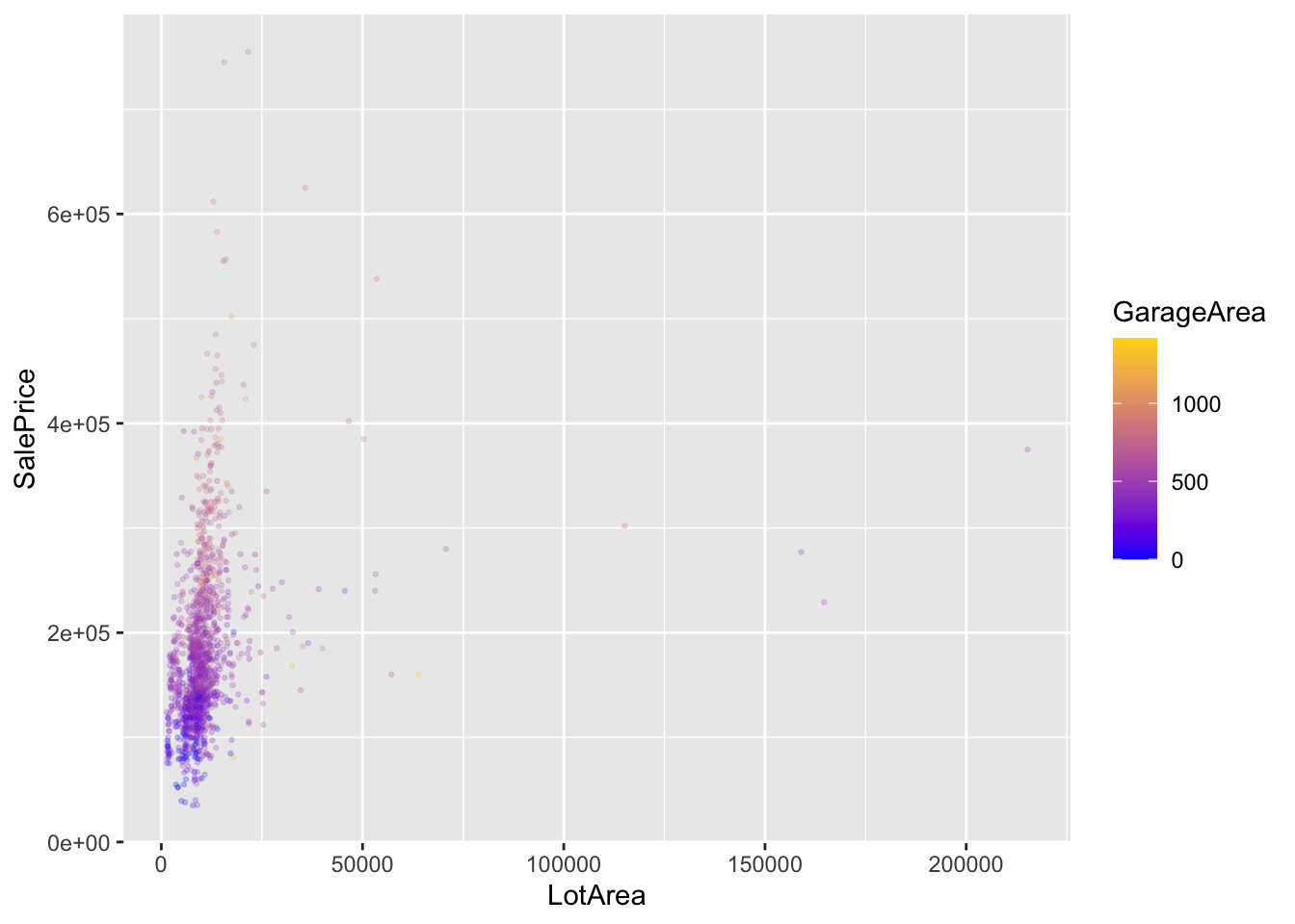
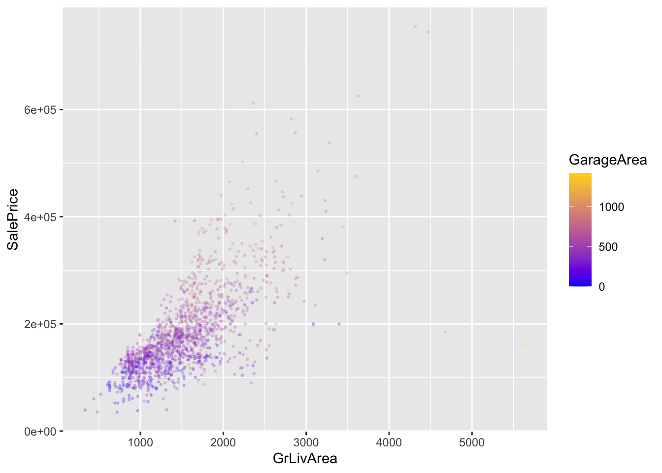
GrLivArea: Above grade (ground) living area square feet

LotArea: Lot size in square feet

GarageArea: Size of garage in square feet

Main effects model:

model_fit = lm(SalePrice ~ LotArea + GarageArea + GrLivArea, 
               data = house_prices)
summary(model_fit)

## 
## Call:
## lm(formula = SalePrice ~ LotArea + GarageArea + GrLivArea, data = house_prices)
## 
## Residuals:
##     Min      1Q  Median      3Q     Max 
## -500375  -22148    -977   19699  315357 
## 
## Coefficients:
##               Estimate Std. Error t value Pr(>|t|)    
## (Intercept) -8031.7724  4154.7983  -1.933 0.053414 .  
## LotArea         0.4821     0.1346   3.582 0.000353 ***
## GarageArea    137.0127     6.8638  19.962  < 2e-16 ***
## GrLivArea      78.5759     2.8472  27.597  < 2e-16 ***
## ---
## Signif. codes:  0 '***' 0.001 '**' 0.01 '*' 0.05 '.' 0.1 ' ' 1
## 
## Residual standard error: 49400 on 1456 degrees of freedom
## Multiple R-squared:  0.6142, Adjusted R-squared:  0.6134 
## F-statistic: 772.6 on 3 and 1456 DF,  p-value: < 2.2e-16

Full model (including also interactions effects):

model_fit = lm(SalePrice ~ LotArea*GarageArea*GrLivArea, 
               data = house_prices)
summary(model_fit)

## 
## Call:
## lm(formula = SalePrice ~ LotArea * GarageArea * GrLivArea, data = house_prices)
## 
## Residuals:
##     Min      1Q  Median      3Q     Max 
## -289270  -20605     590   19121  288645 
## 
## Coefficients:
##                                Estimate Std. Error t value Pr(>|t|)    
## (Intercept)                   8.894e+04  1.229e+04   7.235 7.49e-13 ***
## LotArea                      -2.232e+00  1.166e+00  -1.915  0.05574 .  
## GarageArea                   -9.108e+01  2.109e+01  -4.319 1.68e-05 ***
## GrLivArea                     8.923e+00  7.726e+00   1.155  0.24831    
## LotArea:GarageArea            6.629e-03  1.437e-03   4.614 4.30e-06 ***
## LotArea:GrLivArea             1.935e-03  5.433e-04   3.562  0.00038 ***
## GarageArea:GrLivArea          1.522e-01  1.208e-02  12.599  < 2e-16 ***
## LotArea:GarageArea:GrLivArea -4.305e-06  4.774e-07  -9.016  < 2e-16 ***
## ---
## Signif. codes:  0 '***' 0.001 '**' 0.01 '*' 0.05 '.' 0.1 ' ' 1
## 
## Residual standard error: 45950 on 1452 degrees of freedom
## Multiple R-squared:  0.667,  Adjusted R-squared:  0.6654 
## F-statistic: 415.5 on 7 and 1452 DF,  p-value: < 2.2e-16

# Note: Have main effects changed?

How to visualize it?

ggplot(data = house_prices, aes(x = LotArea, y = SalePrice, color=GarageArea)) +
  geom_jitter(alpha=.2, size=.5) +
  scale_colour_gradient(low = "blue", high = "gold", limits=range(house_prices[,'GarageArea']))

ggplot(data = house_prices, aes(x = GrLivArea, y = SalePrice, color=GarageArea)) +
  geom_jitter(alpha=.2, size=.5) +
  scale_colour_gradient(low = "blue", high = "gold", limits=range(house_prices[,'GarageArea']))

Multicollinearity checks

From the plots above we can see that the predictors are somewhat correlated. But how can we check this best?

M = cor(select(house_prices, LotArea, GarageArea, GrLivArea))
M

##              LotArea GarageArea GrLivArea
## LotArea    1.0000000  0.1804028 0.2631162
## GarageArea 0.1804028  1.0000000 0.4689975
## GrLivArea  0.2631162  0.4689975 1.0000000

To more formally test (bewtween 2 variables):

cor.test(house_prices$GarageArea, house_prices$GrLivArea)

## 
##  Pearson's product-moment correlation
## 
## data:  house_prices$GarageArea and house_prices$GrLivArea
## t = 20.276, df = 1458, p-value < 2.2e-16
## alternative hypothesis: true correlation is not equal to 0
## 95 percent confidence interval:
##  0.4279930 0.5080752
## sample estimates:
##       cor 
## 0.4689975

This means that the assumptions were violated and the coefficients should be interpreted with caution.

Hypothesis tests for all pairwise correlations:

#install.packages("lsr")

library(lsr)

correlate(as.data.frame(select(house_prices, LotArea, GarageArea, GrLivArea)), test=TRUE)

## 
## CORRELATIONS
## ============
## - correlation type:  pearson 
## - correlations shown only when both variables are numeric
## 
##            LotArea    GarageArea    GrLivArea   
## LotArea          .         0.180***     0.263***
## GarageArea   0.180***          .        0.469***
## GrLivArea    0.263***      0.469***         .   
## 
## ---
## Signif. codes: . = p < .1, * = p<.05, ** = p<.01, *** = p<.001
## 
## 
## p-VALUES
## ========
## - total number of tests run:  3 
## - correction for multiple testing:  holm 
## 
##            LotArea GarageArea GrLivArea
## LotArea          .      0.000     0.000
## GarageArea   0.000          .     0.000
## GrLivArea    0.000      0.000         .
## 
## 
## SAMPLE SIZES
## ============
## 
##            LotArea GarageArea GrLivArea
## LotArea       1460       1460      1460
## GarageArea    1460       1460      1460
## GrLivArea     1460       1460      1460

To better visualize the correlation matrix:

#install.packages("corrplot")

library('corrplot')

## corrplot 0.84 loaded

corrplot(M)

Calculating standardised regression coefficients

One more thing that you might want to do is to calculate “standardised” regression coefficients: your predictors are often on different scales and this makes it very difficult to compare the coefficients of different predictors.

The standardised coefficients are the coefficients that you would have obtained if you’d converted all the variables to z-scores before running the regression.

You can then either standardize them first, or use the standardCoefs function in R.

model_fit = lm(SalePrice ~ LotArea+GarageArea+GrLivArea, 
               data = house_prices)
summary(model_fit)

## 
## Call:
## lm(formula = SalePrice ~ LotArea + GarageArea + GrLivArea, data = house_prices)
## 
## Residuals:
##     Min      1Q  Median      3Q     Max 
## -500375  -22148    -977   19699  315357 
## 
## Coefficients:
##               Estimate Std. Error t value Pr(>|t|)    
## (Intercept) -8031.7724  4154.7983  -1.933 0.053414 .  
## LotArea         0.4821     0.1346   3.582 0.000353 ***
## GarageArea    137.0127     6.8638  19.962  < 2e-16 ***
## GrLivArea      78.5759     2.8472  27.597  < 2e-16 ***
## ---
## Signif. codes:  0 '***' 0.001 '**' 0.01 '*' 0.05 '.' 0.1 ' ' 1
## 
## Residual standard error: 49400 on 1456 degrees of freedom
## Multiple R-squared:  0.6142, Adjusted R-squared:  0.6134 
## F-statistic: 772.6 on 3 and 1456 DF,  p-value: < 2.2e-16

standardCoefs(model_fit)

##                      b       beta
## LotArea      0.4820601 0.06056669
## GarageArea 137.0127177 0.36874445
## GrLivArea   78.5759048 0.51974818

house_prices = mutate(house_prices,
                      z_LotArea = scale(LotArea, center = TRUE, scale = TRUE),
                      z_GarageArea = scale(GarageArea, center = TRUE, scale = TRUE),
                      z_GrLivArea = scale(GrLivArea, center = TRUE, scale = TRUE),
                      z_SalePrice = scale(SalePrice, center = TRUE, scale = TRUE))

st_model_fit = lm(z_SalePrice ~ z_LotArea+z_GarageArea+z_GrLivArea, 
               data = house_prices)
summary(st_model_fit)

## 
## Call:
## lm(formula = z_SalePrice ~ z_LotArea + z_GarageArea + z_GrLivArea, 
##     data = house_prices)
## 
## Residuals:
##     Min      1Q  Median      3Q     Max 
## -6.2986 -0.2788 -0.0123  0.2480  3.9696 
## 
## Coefficients:
##               Estimate Std. Error t value Pr(>|t|)    
## (Intercept)  1.779e-16  1.627e-02   0.000 1.000000    
## z_LotArea    6.057e-02  1.691e-02   3.582 0.000353 ***
## z_GarageArea 3.687e-01  1.847e-02  19.962  < 2e-16 ***
## z_GrLivArea  5.197e-01  1.883e-02  27.597  < 2e-16 ***
## ---
## Signif. codes:  0 '***' 0.001 '**' 0.01 '*' 0.05 '.' 0.1 ' ' 1
## 
## Residual standard error: 0.6218 on 1456 degrees of freedom
## Multiple R-squared:  0.6142, Adjusted R-squared:  0.6134 
## F-statistic: 772.6 on 3 and 1456 DF,  p-value: < 2.2e-16

What happened now to the intercept?

2. ANOVA

General linear models

We use linear regression models when we want to predict a continuous variable based on one or more continuous variables, assuming a linear relationship.

But we can also predict a continuous variable based on one or more categorical variables using the ANOVA.

Both linear regression and ANOVA, however, are part of the same category of models: general linear models.

The general linear model or multivariate regression model is a statistical linear model. It may be written as:

Y = XB + U,

where: - Y is a matrix with series of multivariate measurements (each column being a set of measurements on one of the dependent variables), - X is a matrix of observations on independent variables that might be a design matrix (each column being a set of observations on one of the independent variables), - B is a matrix containing parameters that are usually to be estimated - and U is a matrix containing errors (noise). The errors are usually assumed to be uncorrelated across measurements, and follow a multivariate normal distribution.

The general linear model incorporates a number of different statistical models: ANOVA, ANCOVA, MANOVA, MANCOVA, ordinary linear regression, t-test and F-test.

When to use ANOVA/linear regression?

In practice, we use Analysis of variance (ANOVA) when we have categorical-only predictors. As soon as we have at least one continuous predictor we would switch to linear regression.

The conversion between ANOVA and regression depends on how we code the categorical predictors (see here for a clear example).

Different types of ANOVAS

• One-way ANOVA is used to test for differences among two or more independent groups (means), e.g., different levels of urea application in a crop, or different levels of antibiotic action on several different bacterial species, or different levels of effect of some medicine on groups of patients.

• However, should these groups not be independent, and there is an order in the groups (such as mild, moderate and severe disease), or in the dose of a drug (such as 5 mg/mL, 10 mg/mL, 20 mg/mL) given to the same group of patients, then a linear trend estimation should be used. Typically, however, the one-way ANOVA is used to test for differences among at least three groups, since the two-group case can be covered by a t-test. When there are only two means to compare, the t-test and the ANOVA F-test are equivalent; the relation between ANOVA and t is given by F = t2.

• Two-way ANOVA is an extension of the one-way ANOVA that examines the influence of two different categorical independent variables on one continuous dependent variable. The two-way ANOVA not only aims at assessing the main effect of each independent variable but also if there is any interaction between them.

• Repeated measures ANOVA is used when the same subjects are used for each treatment (e.g., in a longitudinal study).

• Multivariate analysis of variance (MANOVA) is used when there is more than one response variable.

ANOVA’s assumptions

Because ANOVA and linear regression are essentially the same (see better explanations above), the model’s assumptions are also very similar:

• Normality: The residuals are assumed to be normally distributed. As we saw for linear regression, we can assess this by looking at QQ plots or running a Shapiro-Wilk test.
• Homogeneity of variance (homoscedasticity): ANOVA assumes that the population standard deviation is the same for all groups. We can assess this using the Levene’s test (see below) and visually using a violin or similar plots.
• Independence: the observations should be independent. In case of repeated measures study, you should then use the repeated measure ANOVA (that we don’t cover in this course).

Model checking and fitting

To fit ANOVAs, we use the aov() function.

This function works very similarly to the lm() function: you need a formula argument and a data argument to make it work.

sub_house_prices = filter(house_prices, Foundation == "Slab" | Foundation == "Stone" | Foundation == "Wood")

arrange(summarize(group_by(sub_house_prices, Foundation),
          mean_SalePrice = mean(SalePrice),
          sd_SalePrice = sd(SalePrice)),
        mean_SalePrice)

## # A tibble: 3 x 3
##   Foundation mean_SalePrice sd_SalePrice
##   <chr>               <dbl>        <dbl>
## 1 Slab              107366.       34214.
## 2 Stone             165959.       78558.
## 3 Wood              185667.       56695.

ggplot(data = sub_house_prices, mapping = aes(y = SalePrice, x = Foundation)) +
  geom_violin()

Note that you can also here check whether the normality assumption is violated or not. You can do so by also plotting separate histograms per level of your categorical variable.

More formally:

shapiro.test(filter(sub_house_prices, Foundation == "Slab")$SalePrice)

## 
##  Shapiro-Wilk normality test
## 
## data:  filter(sub_house_prices, Foundation == "Slab")$SalePrice
## W = 0.94837, p-value = 0.2498

shapiro.test(filter(sub_house_prices, Foundation == "Stone")$SalePrice)

## 
##  Shapiro-Wilk normality test
## 
## data:  filter(sub_house_prices, Foundation == "Stone")$SalePrice
## W = 0.74492, p-value = 0.01776

shapiro.test(filter(sub_house_prices, Foundation == "Wood")$SalePrice)

## 
##  Shapiro-Wilk normality test
## 
## data:  filter(sub_house_prices, Foundation == "Wood")$SalePrice
## W = 0.89046, p-value = 0.3558

Levene’s test of equal variance: Low p-value means the variances are not equal.

For the test of equal variances, we need a package called car.

The first argument in the function is thr continuous dependent variable, the second argument is the categorical independent variable.

#install.packages("car")

library(car)

## Loading required package: carData

## Registered S3 methods overwritten by 'car':
##   method                          from
##   influence.merMod                lme4
##   cooks.distance.influence.merMod lme4
##   dfbeta.influence.merMod         lme4
##   dfbetas.influence.merMod        lme4

## 
## Attaching package: 'car'

## The following object is masked from 'package:dplyr':
## 
##     recode

## The following object is masked from 'package:purrr':
## 
##     some

leveneTest(sub_house_prices$SalePrice, sub_house_prices$Foundation) 

## Warning in leveneTest.default(sub_house_prices$SalePrice, sub_house_prices$Foundation): sub_house_prices$Foundation
## coerced to factor.

## Levene's Test for Homogeneity of Variance (center = median)
##       Df F value Pr(>F)
## group  2  2.0824 0.1423
##       30

Finally, the actual ANOVA:

model_fit = aov(SalePrice ~ Foundation, 
                data = sub_house_prices)
summary(model_fit)

##             Df    Sum Sq   Mean Sq F value Pr(>F)   
## Foundation   2 2.857e+10 1.428e+10   6.674  0.004 **
## Residuals   30 6.421e+10 2.140e+09                  
## ---
## Signif. codes:  0 '***' 0.001 '**' 0.01 '*' 0.05 '.' 0.1 ' ' 1

print(model_fit)

## Call:
##    aov(formula = SalePrice ~ Foundation, data = sub_house_prices)
## 
## Terms:
##                  Foundation   Residuals
## Sum of Squares  28569939851 64208950589
## Deg. of Freedom           2          30
## 
## Residual standard error: 46263.36
## Estimated effects may be unbalanced

Tukey’s honest significant difference test

Note that ANOVA tests the null hypothesis that the means in all our groups are equal. A rejection of this null hypothesis means that there is a significant difference in at least one of the possible pairs of means.

To get an idea of which pair of means contains a significant difference, we can follow up with Tukey’s test that will give us all pairwise comparisons.

Tukey’s test corrects the p-values upwards — so it is more conservative in deciding something is significant — because the comparisons are post-hoc or exploratory:

TukeyHSD(model_fit, "Foundation")

##   Tukey multiple comparisons of means
##     95% family-wise confidence level
## 
## Fit: aov(formula = SalePrice ~ Foundation, data = sub_house_prices)
## 
## $Foundation
##                diff        lwr      upr     p adj
## Stone-Slab 58593.54   6536.288 110650.8 0.0247988
## Wood-Slab  78301.04   8458.907 148143.2 0.0254424
## Wood-Stone 19707.50 -60939.251 100354.3 0.8198692

3. Now it’s your turn

Student Performance

From github, get the student-mat.csv and student-por.csv datasets.

Task A

1. Using the student_math dataset, create a regression object called model_fit_1 predicting third period grade (G3) based on sex, age, internet, and failures. How do you interpret the regression output? Which variables are significantly related to third period grade?

2. Check the model’s assumptions. Which are violated?

3. Load the student-por.csv in R as student_port. Inspect the dataset first.

4. Create a new regression object called model_fit_2 using the same variables as question 1: however, this time use the portugese dataset.

5. What are the key differences between the beta values for the portugese dataset (model_fit_2) and the math dataset (model_fit_1)?

Task B

1. Using the student_math dataset, create a regression object called model_fit_3 predicting first period grade (G1) based on guardian. Guardian is a nominal variable with 3 levels.

2. Use summary to look at the output. You should see 2 predictors listed (“guardianmother” and “guardiananother”), rather than the expected 1 (“guardian”). lm has dummy coded your variables with “father” set as the reference group. Look at the levels of the guardian factor to see why “father” is the reference group. How would you interpret the results?

3. What is the predicted grade for those with a father as their guardian? Those with a mother? Those with other? Compare these to the means of each group again.

Task C

1. Using the student_math dataset, create a regression object called model_fit_4 predicting a student’s first period grade (G1) based on all variables in the dataset (Hint: use the notation formula = y ~ . to include all variables)

2. Save the fitted values from the model_fit_4 object as a vector called model_4_fitted.

3. Using the student_math dataset, create a scatterplot showing the relationship between a student’s first period grade (G1) and the fitted values from the model. Does the model appear to correctly fit a student’s first period grade? Use geom_abline() with slope=1 and intercept=0 to plot the identity line and better answer to this question.

4. Create a new regression object, called model_fit_5 which doesn’t include G2 or G3 as predictors, but still includes all other variables. Save the fitted values from the model_fit_5 object as a vector called model_5_fitted.

5. Plot the predicted grades against the actual ones, as predicted by model model_fit_5, as in question 3. How well does the new model perform now?

Task D

• For each question, conduct the appropriate ANOVA. Write the conclusion in APA style. To summarize an effect in an ANOVA, use the format F(XXX, YYY) = FFF, p = PPP, where XXX is the degrees of freedom of the variable you are testing, YYY is the degrees of freedom of the residuals, FFF is the F value for the variable you are testing, and PPP is the p-value. If the p-value is less than .01, just write p < .01.

• For the purposes of this class, if the p-value of the ANOVA is less than .05, conduct post-hoc tests. If you are only testing one independent variable, write APA conclusions for the post-hoc test. If you are testing more than one independent variable in your ANOVA, you do not need to write APA style conclusions for post-hoc tests – just comment the result.

For example, here is how you would analyze and answer the question: “Was there an effect of diets on Chicken Weights?””

# ANOVA on Chicken Weights
#   IV = Diet, DV = weight

# ANOVA
model_fit = aov(formula = weight ~ Diet, data = ChickWeight)

summary(model_fit)

# ANOVA was significant (p < .01), so I'll conduct post-hoc tests

# Tukey post-hoc tests
TukeyHSD(model_fit)

# There was a significant main effect of diets on chicken weights (F(3, 574) = 10.81, p < .01). 
# Pairwise Tukey HSD tests showed significant differences between diets 1 and 3 (diff = 40.30, p < .01) 
# and diets 1 and 4 (diff = 32.62, p < .01). 
# All other pairwise differences were not significant at the 0.05 significance threshold.

1. Using the student_math dataset, was there a main effect of the school support on G1? Conduct a one-way ANOVA. If the result is significant (p < .05), conduct post-hoc tests.

2. Using the student_math dataset, was there a main effect of the family support on G1? Conduct a one-way ANOVA. If the result is significant (p < .05), conduct post-hoc tests.

3. Conduct a two-way ANOVA on G1 with both school support and family support as IVs. Do your results for each variable change compared to your previous one-way ANOVAs on these variables? (You do not need to give APA results or conduct post-hoc tests, just answer the question verbally).

Submit your assignment

Save and email your script to me at laura.fontanesi@unibas.ch by the end of Friday.