Solutions to WPA4
6. Now it’s your turn
Now you will analyze data from Matthews et al. (2016): Why do we overestimate others’ willingness to pay? The purpose of this research was to test if our beliefs about other people’s affluence (i.e.; wealth) affect how much we think they will be willing to pay for items. You can find the full paper at http://journal.sjdm.org/15/15909/jdm15909.pdf.
Variables description:
Here are descriptions of the data variables (taken from the author’s dataset notes available at http://journal.sjdm.org/15/15909/Notes.txt)
id: participant id codegender: participant gender. 1 = male, 2 = femaleage: participant ageincome: participant annual household income on categorical scale with 8 categorical options: Less than 5,000; 15,001–25,000; 25,001–35,000; 35,001–50,000; 50,001–75,000; 75,001–100,000; 100,001–150,000; greater than 150,000.p1-p10: whether the “typical” survey respondent would pay more (coded 1) or less (coded 0) than oneself, for each of the 10 productstask: whether the participant had to judge the proportion of other people who “have more money than you do” (coded 1) or the proportion who “have less money than you do” (coded 0)havemore: participant’s response when task = 1haveless: participant’s response when task = 0pcmore: participant’s estimate of the proportion of people who have more than they do (calculated as 100-haveless when task=0)
Task A
First, download the data_wpa4.csv and
matthews_demographics.csv datasets from the data
folder on Github and load them in R.
library(tidyverse)

matthews_data = read_csv('https://raw.githubusercontent.com/laurafontanesi/r-seminar22/master/data/data_wpa4.csv')
##
## ── Column specification ─────────────────────────────────────────────────────────────────────────────────────────────
## cols(
## id = col_character(),
## gender = col_double(),
## age = col_double(),
## income = col_double(),
## p1 = col_double(),
## p2 = col_double(),
## p3 = col_double(),
## p4 = col_double(),
## p5 = col_double(),
## p6 = col_double(),
## p7 = col_double(),
## p8 = col_double(),
## p9 = col_double(),
## p10 = col_double(),
## task = col_double(),
## havemore = col_double(),
## haveless = col_double(),
## pcmore = col_double()
## )demographics = read_csv("https://raw.githubusercontent.com/laurafontanesi/r-seminar22/master/data/matthews_demographics.csv")## Warning: Missing column names filled in: 'X1' [1]##
## ── Column specification ─────────────────────────────────────────────────────────────────────────────────────────────
## cols(
## X1 = col_double(),
## id = col_character(),
## height = col_double(),
## race = col_character()
## )glimpse(matthews_data)## Rows: 190
## Columns: 18
## $ id <chr> "R_3PtNn51LmSFdLNM", "R_2AXrrg62pgFgtMV", "R_cwEOX3HgnMeVQHL", "R_d59iPwL4W6BH8qx", "R_1f3K2HrGzFG…
## $ gender <dbl> 2, 2, 1, 1, 1, 1, 1, 1, 1, 1, 1, 1, 1, 2, 1, 2, 2, 2, 2, 1, 2, 2, 1, 1, 2, 2, 1, 2, 2, 1, 1, 2, 1,…
## $ age <dbl> 26, 32, 25, 33, 24, 22, 47, 26, 29, 32, 29, 28, 31, 24, 25, 28, 20, 41, 44, 23, 49, 26, 19, 57, 30…
## $ income <dbl> 7, 4, 2, 5, 1, 2, 3, 4, 1, 7, 4, 3, 2, 2, 6, 3, 2, 2, 1, 3, 3, 6, 4, 5, 5, 2, 3, 2, 5, 4, 6, 7, 5,…
## $ p1 <dbl> 1, 1, 0, 1, 1, 1, 1, 1, 1, 1, 1, 1, 0, 1, 1, 0, 1, 1, 1, 1, 0, 0, 1, 0, 0, 1, 0, 1, 0, 1, 1, 1, 1,…
## $ p2 <dbl> 1, 1, 1, 1, 1, 1, 1, 1, 1, 1, 1, 1, 0, 1, 0, 1, 1, 1, 1, 1, 1, 0, 1, 1, 1, 1, 1, 1, 1, 1, 1, 0, 1,…
## $ p3 <dbl> 1, 1, 1, 1, 0, 0, 0, 0, 0, 1, 1, 0, 0, 1, 0, 1, 0, 1, 1, 1, 1, 0, 1, 1, 1, 1, 0, 1, 1, 1, 1, 0, 1,…
## $ p4 <dbl> 1, 1, 1, 1, 1, 0, 0, 0, 1, 1, 1, 1, 1, 1, 1, 1, 1, 1, 1, 1, 1, 1, 1, 0, 1, 1, 1, 1, 1, 1, 1, 0, 1,…
## $ p5 <dbl> 1, 1, 1, 1, 1, 1, 1, 0, 0, 1, 1, 0, 0, 1, 1, 1, 1, 1, 1, 1, 1, 1, 1, 0, 1, 1, 1, 1, 1, 1, 1, 0, 1,…
## $ p6 <dbl> 1, 1, 1, 1, 1, 1, 1, 1, 1, 1, 1, 0, 1, 1, 0, 1, 1, 0, 1, 1, 1, 1, 1, 1, 1, 1, 1, 1, 1, 1, 0, 1, 1,…
## $ p7 <dbl> 1, 1, 1, 1, 1, 1, 1, 1, 1, 1, 1, 1, 1, 1, 1, 1, 0, 1, 1, 1, 0, 0, 1, 1, 1, 1, 1, 1, 1, 1, 0, 0, 1,…
## $ p8 <dbl> 1, 1, 1, 1, 1, 1, 1, 1, 1, 0, 1, 1, 1, 1, 1, 1, 1, 1, 1, 1, 1, 1, 1, 1, 1, 1, 1, 1, 1, 1, 1, 1, 1,…
## $ p9 <dbl> 1, 1, 0, 1, 1, 0, 1, 0, 1, 1, 1, 0, 1, 1, 1, 1, 1, 1, 1, 1, 1, 0, 0, 0, 0, 1, 1, 1, 0, 1, 0, 0, 1,…
## $ p10 <dbl> 1, 1, 0, 1, 1, 1, 0, 0, 1, 1, 1, 0, 1, 1, 0, 1, 0, 1, 1, 0, 1, 0, 1, 1, 0, 1, 1, 1, 1, 1, 1, 1, 1,…
## $ task <dbl> 0, 0, 0, 0, 1, 0, 1, 0, 1, 1, 1, 1, 0, 0, 0, 1, 0, 0, 1, 0, 1, 1, 0, 1, 1, 0, 1, 1, 0, 1, 1, 1, 0,…
## $ havemore <dbl> NA, NA, NA, NA, 99, NA, 95, NA, 70, 25, 50, 50, NA, NA, NA, 95, NA, NA, 85, NA, 45, 25, NA, 50, 50…
## $ haveless <dbl> 50, 25, 10, 50, NA, 20, NA, 30, NA, NA, NA, NA, 44, 20, 65, NA, 50, 2, NA, 85, NA, NA, 25, NA, NA,…
## $ pcmore <dbl> 50, 75, 90, 50, 99, 80, 95, 70, 70, 25, 50, 50, 56, 80, 35, 95, 50, 98, 85, 15, 45, 25, 75, 50, 50…glimpse(demographics)## Rows: 190
## Columns: 4
## $ X1 <dbl> 1, 2, 3, 4, 5, 6, 7, 8, 9, 10, 11, 12, 13, 14, 15, 16, 17, 18, 19, 20, 21, 22, 23, 24, 25, 26, 27, 2…
## $ id <chr> "R_2zOA03wY3kZPHKj", "R_1f30AbYQR0D1wpt", "R_2YgEERKijE2Hz6K", "R_1CdL2n22srUR26d", "R_1HnsqBRimnKph…
## $ height <dbl> 182, 184, 175, 177, 187, 178, 168, 193, 180, 159, 160, 172, 165, 162, 169, 169, 167, 168, 178, 167, …
## $ race <chr> "black", "white", "hispanic", "white", "white", "white", "white", "white", "white", "hispanic", "whi…Note: do not use pipes from 1 to 4.
- Currently
genderis coded as 1 and 2. Create a new dataframe callednew_matthews_data, in which there is a new column calledgender_labelsthat codes gender as “male” and “female”. Do it usingmutate. Then, rename the originalgendercolumn togender_binaryusingrename. Subtract 1 to all values ofgender_binary, so that it is coded as 0 and 1 instead of 1 and 2 usingmutateagain.
new_matthews_data = mutate(matthews_data,
                           gender_labels = recode(gender,
                                                  `1`="male",
                                                  `2`="female"))
new_matthews_data = rename(new_matthews_data,
                           gender_binary = gender)

new_matthews_data = mutate(new_matthews_data,
                           gender_binary = gender_binary - 1)
head(select(new_matthews_data, gender_binary, gender_labels))
## # A tibble: 6 x 2
## gender_binary gender_labels
## <dbl> <chr>
## 1 1 female
## 2 1 female
## 3 0 male
## 4 0 male
## 5 0 male
## 6 0 male- In
new_matthews_data, create new column calledincome_labelsthat codes income based on the data description above usingmutate. Then, create a new column, calledincome_recoded, where you only have 4 income categories (coded as numbers from 1 to 4): below 25,000, 25,000-50,000, 50,000-100,000, and above 100,000 usingcase_when. How many observations are there for each of these 4 categories? Usesummariseto reply.
new_matthews_data = mutate(new_matthews_data,
                           income_lables = recode(income,
                                                  `1`='less5,000',
                                                  `2`='15,001–25,000',
                                                  `3`='25,001–35,000',
                                                  `4`='35,001–50,000',
                                                  `5`='50,001–75,000',
                                                  `6`='75,001–100,000',
                                                  `7`='100,001–150,000',
                                                  `8`='greater150,000'
                                                 ),
                           income_recoded = case_when(income < 3 ~ 1,
                                                      income >=3 & income < 5 ~ 2,
                                                      income >= 5 & income < 7 ~ 3,
                                                      income >=7 ~ 4))

summarise(group_by(new_matthews_data, income_recoded),
          n = n())
## # A tibble: 4 x 2
## income_recoded n
## <dbl> <int>
## 1 1 72
## 2 2 56
## 3 3 52
## 4 4 10- In
new_matthews_data, transform all numeric columns into integers numbers usingmutate_if.
new_matthews_data = mutate_if(new_matthews_data,
                              is.numeric,
                              as.integer)
head(new_matthews_data)
## # A tibble: 6 x 21
## id gender_binary age income p1 p2 p3 p4 p5 p6 p7 p8 p9 p10 task havemore
## <chr> <int> <int> <int> <int> <int> <int> <int> <int> <int> <int> <int> <int> <int> <int> <int>
## 1 R_3PtNn51LmS… 1 26 7 1 1 1 1 1 1 1 1 1 1 0 NA
## 2 R_2AXrrg62pg… 1 32 4 1 1 1 1 1 1 1 1 1 1 0 NA
## 3 R_cwEOX3HgnM… 0 25 2 0 1 1 1 1 1 1 1 0 0 0 NA
## 4 R_d59iPwL4W6… 0 33 5 1 1 1 1 1 1 1 1 1 1 0 NA
## 5 R_1f3K2HrGzF… 0 24 1 1 1 0 1 1 1 1 1 1 1 1 99
## 6 R_3oN5ijzTfo… 0 22 2 1 1 0 0 1 1 1 1 0 1 0 NA
## # … with 5 more variables: haveless <int>, pcmore <int>, gender_labels <chr>, income_lables <chr>,
## # income_recoded <int>- From
new_matthews_data, create a summary of the dataset usingsummarise, to answer the following questions: What percent of participants were female? What was the minimum, mean, and maximumincome? What was the 25th percentile, median, and the 75th percentile ofage? Use good names for columns.
summarise(new_matthews_data,
          perc_female = mean(gender_binary)*100,
          min_income = min(income),
          mean_income = mean(income),
          max_income = max(income),
          perc25_age = quantile(age, .25),
          median_age = quantile(age, .5),
          perc75_age = quantile(age, .75)
          )
## # A tibble: 1 x 7
## perc_female min_income mean_income max_income perc25_age median_age perc75_age
## <dbl> <int> <dbl> <int> <dbl> <dbl> <dbl>
## 1 37.4 1 3.53 8 25 30 35- Repeat steps from 1 to 4 (apart from the
summarisein point 2) using pipes and assign the result tonew_matthews_data_summary.
new_matthews_data_summary = matthews_data %>%
    mutate(gender_labels = recode(gender,
                                 `1`="male",
                                 `2`="female"))  %>%
    rename(gender_binary = gender)  %>%
    mutate(gender_binary = gender_binary - 1) %>%
    mutate(income_lables = recode(income,
                                  `1`='less5,000',
                                  `2`='15,001–25,000',
                                  `3`='25,001–35,000',
                                  `4`='35,001–50,000',
                                  `5`='50,001–75,000',
                                  `6`='75,001–100,000',
                                  `7`='100,001–150,000',
                                  `8`='greater150,000'),
           income_recoded = case_when(income < 3 ~ 1,
                                      income >=3 & income < 5 ~ 2,
                                      income >= 5 & income < 7 ~ 3,
                                      income >=7 ~ 4)) %>%
    mutate_if(is.numeric,
              as.integer) %>%
    summarise(perc_female = mean(gender_binary)*100,
              min_income = min(income),
              mean_income = mean(income),
              max_income = max(income),
              perc25_age = quantile(age, .25),
              median_age = quantile(age, .5),
              perc75_age = quantile(age, .75))

print(new_matthews_data_summary)
## # A tibble: 1 x 7
## perc_female min_income mean_income max_income perc25_age median_age perc75_age
## <dbl> <int> <dbl> <int> <dbl> <dbl> <dbl>
## 1 37.4 1 3.53 8 25 30 35Task B
- From
new_matthews_data, calculate the meanp1top10across participants usingsummarise_allandselect. Which product scored the highest? Do it again, grouping the data by gender. Is there a difference across gender? What is the mean of the meanp1top10across participants? Calculate it on the result of the previous step. You can do these either using pipes or not.
# with pipes
new_matthews_data %>%
    group_by(gender_binary) %>%
    select(p1:p10) %>%
    summarise_all(mean)
## Adding missing grouping variables: `gender_binary`## # A tibble: 2 x 11
## gender_binary p1 p2 p3 p4 p5 p6 p7 p8 p9 p10
## <int> <dbl> <dbl> <dbl> <dbl> <dbl> <dbl> <dbl> <dbl> <dbl> <dbl>
## 1 0 0.723 0.849 0.630 0.857 0.790 0.782 0.866 0.874 0.689 0.706
## 2 1 0.648 0.887 0.831 0.845 0.746 0.831 0.859 0.944 0.648 0.775# without pipes
selected_data = select(new_matthews_data, p1:p10, gender_binary)
grouped_data = group_by(selected_data, gender_binary)
summarise_all(grouped_data, mean)## # A tibble: 2 x 11
## gender_binary p1 p2 p3 p4 p5 p6 p7 p8 p9 p10
## <int> <dbl> <dbl> <dbl> <dbl> <dbl> <dbl> <dbl> <dbl> <dbl> <dbl>
## 1 0 0.723 0.849 0.630 0.857 0.790 0.782 0.866 0.874 0.689 0.706
## 2 1 0.648 0.887 0.831 0.845 0.746 0.831 0.859 0.944 0.648 0.775- Transform the data from wide to long format. In particular, you want
10 rows per subjects, with their responses on the products 1 to 10 in a
column called
wtp, and the product label in a column calledproduct. Call the resulting dataframenew_matthews_data_long. Re-order it byid. Print the first 20 cases to check this worked. Check thatnew_matthews_data_longhas 10 times more rows thannew_matthews_data.
# these are the solutions for B2, as we will cover wide to long data transformation later in the seminar
new_matthews_data_long = gather(new_matthews_data,
                                key='product',
                                value='wtp',
                                p1:p10)

new_matthews_data_long = arrange(new_matthews_data_long, id)

head(new_matthews_data_long)
## # A tibble: 6 x 13
## id gender_binary age income task havemore haveless pcmore gender_labels income_lables income_recoded product
## <chr> <int> <int> <int> <int> <int> <int> <int> <chr> <chr> <int> <chr>
## 1 R_0JL… 1 45 4 1 80 NA 80 female 35,001–50,000 2 p1
## 2 R_0JL… 1 45 4 1 80 NA 80 female 35,001–50,000 2 p2
## 3 R_0JL… 1 45 4 1 80 NA 80 female 35,001–50,000 2 p3
## 4 R_0JL… 1 45 4 1 80 NA 80 female 35,001–50,000 2 p4
## 5 R_0JL… 1 45 4 1 80 NA 80 female 35,001–50,000 2 p5
## 6 R_0JL… 1 45 4 1 80 NA 80 female 35,001–50,000 2 p6
## # … with 1 more variable: wtp <int>Task C
- Drop the
X1column indemographicsusingselect.
demographics = select(demographics, -c(X1))

head(demographics)
## # A tibble: 6 x 3
## id height race
## <chr> <dbl> <chr>
## 1 R_2zOA03wY3kZPHKj 182 black
## 2 R_1f30AbYQR0D1wpt 184 white
## 3 R_2YgEERKijE2Hz6K 175 hispanic
## 4 R_1CdL2n22srUR26d 177 white
## 5 R_1HnsqBRimnKphfg 187 white
## 6 R_12PUXbJhfNF9GAE 178 white- Join
new_matthews_data_longanddemographicsbased on theid, in order to retain as many rows and columns as possible. Call the resulting dataframematthews_data_all.
matthews_data_all = full_join(new_matthews_data_long, demographics, by="id")

head(matthews_data_all)
## # A tibble: 6 x 15
## id gender_binary age income task havemore haveless pcmore gender_labels income_lables income_recoded product
## <chr> <int> <int> <int> <int> <int> <int> <int> <chr> <chr> <int> <chr>
## 1 R_0JL… 1 45 4 1 80 NA 80 female 35,001–50,000 2 p1
## 2 R_0JL… 1 45 4 1 80 NA 80 female 35,001–50,000 2 p2
## 3 R_0JL… 1 45 4 1 80 NA 80 female 35,001–50,000 2 p3
## 4 R_0JL… 1 45 4 1 80 NA 80 female 35,001–50,000 2 p4
## 5 R_0JL… 1 45 4 1 80 NA 80 female 35,001–50,000 2 p5
## 6 R_0JL… 1 45 4 1 80 NA 80 female 35,001–50,000 2 p6
## # … with 3 more variables: wtp <int>, height <dbl>, race <chr>- Calculate the mean
wtpper subject usinggroup_by. You can use pipes or not. Called the resulting dataframemean_matthews_data_all. This should have as many rows as the number of subjects and 2 columns (idand mean wtp). Add as a third and fourth columnsheigthandraceusing one of the join functions.
mean_matthews_data_all = matthews_data_all %>%
    group_by(id) %>%
    summarise(mean_wtp=mean(wtp))

mean_matthews_data_all = full_join(mean_matthews_data_all, demographics, by="id")

head(mean_matthews_data_all)
## # A tibble: 6 x 4
## id mean_wtp height race
## <chr> <dbl> <dbl> <chr>
## 1 R_0JLtfRpOyh8pOCN 0.9 176 black
## 2 R_0O52mja29pBTphb 0.6 171 asian
## 3 R_0OnZ5ZwmVAU6w2V 0.8 150 hispanic
## 4 R_0oXJeSTrYNzQlRH 0.8 180 asian
## 5 R_10CVQqqmFiczGPS 0.7 173 asian
## 6 R_10HKEOMi0HhWe7T 0.7 177 asian- Using
mean_matthews_data_all, make a barplot showing the meanwtpacross ethnic groups. Plot confidence intervals. Give appropriate labels to the plot. Do you think there is a difference in willingness to pay across groups?
# these are the solutions for B4, as we will cover plotting later in the seminar
ggplot(data = mean_matthews_data_all, mapping = aes(x = factor(race), y = mean_wtp)) +
    stat_summary(fun = "mean", geom="bar") +
    stat_summary(fun.data = mean_cl_normal, geom = "errorbar", size=1, width=.4) +
    labs(x = 'Race', y = 'Mean WTP') +
    theme(axis.text.x = element_text(angle = 90))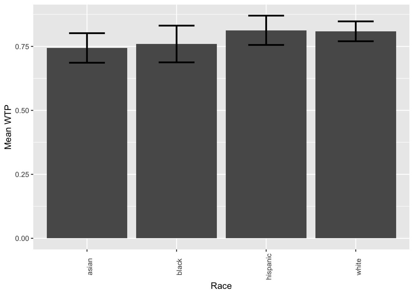
- Using
mean_matthews_data_all, make a scatterplot showing the wtp on the y-axis and the height on the x-axis. Add a regression line. Do you think height predicts willingness to pay?
# these are the solutions for B5, as we will cover plotting later in the seminar
ggplot(data = mean_matthews_data_all, mapping = aes(x = height, y = mean_wtp)) +
    geom_point(alpha = 0.3, size= 2) +
    geom_smooth(method = lm, color='grey') +
    labs(x='Height', y='Mean WTP') +
    ggtitle("Relationship betweenheight and WTP")
## `geom_smooth()` using formula 'y ~ x'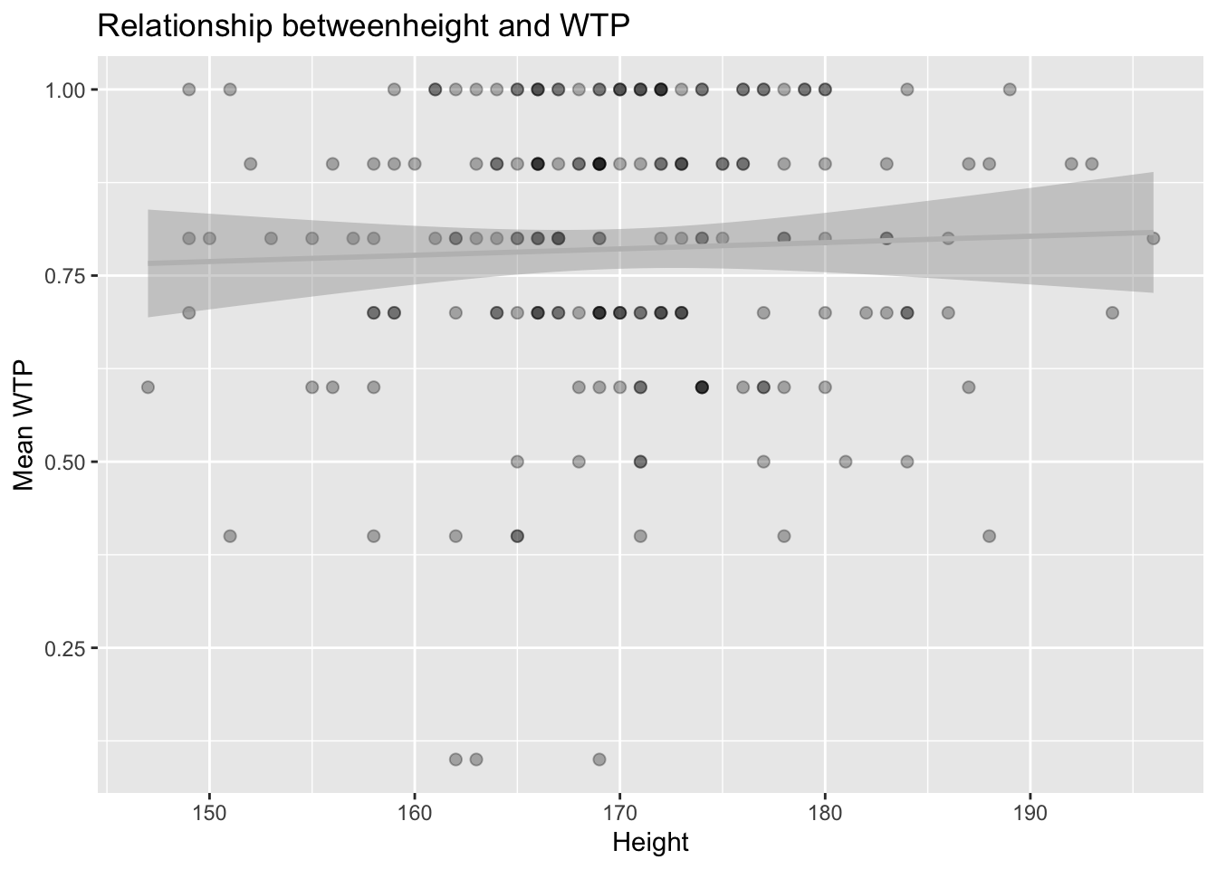
Submit your assignment
Save and email your script to me at laura.fontanesi@unibas.ch by the end of Friday.