The race diffusion model
rm(list = ls())
library(tidyverse)
library(dfoptim)
library(rtdists)
library(rstan)
library(bayesplot)
source('rwald code.r') # from https://osf.io/3sp9t/
We can write down Equation 1 of the Tillman paper to simulate the process described by the race diffusion model:
rdm_path <- function(drift1, drift2, threshold, ndt, sp1=0, sp2=0, noise_constant=1, dt=0.001, max_rt=10) {
  max_tsteps <- max_rt/dt

  # initialize the diffusion process
  tstep <- 0
  x1 <- c(sp1*threshold) # vector of accumulated evidence at t=tstep
  x2 <- c(sp2*threshold) # vector of accumulated evidence at t=tstep
  time <- c(ndt)

  # start accumulating
  while (x1[tstep+1] < threshold & x2[tstep+1] < threshold & tstep < max_tsteps) {
    x1 <- c(x1, x1[tstep+1] + rnorm(mean=drift1*dt, sd=noise_constant*sqrt(dt), n=1))
    x2 <- c(x2, x2[tstep+1] + rnorm(mean=drift2*dt, sd=noise_constant*sqrt(dt), n=1))
    time <- c(time, dt*tstep + ndt)
    tstep <- tstep + 1
  }
  return (data.frame(time=rep(time, 2), dv=c(x1, x2), accumulator=c(rep(1, length(x1)), rep(2, length(x2)))))
}
And visualize it:
gen_drift1 = 1.7
gen_drift2 = 2
gen_threshold = 1
gen_ndt = .23
sim_path <- rdm_path(gen_drift1, gen_drift2, gen_threshold, gen_ndt)

ggplot(data = sim_path, aes(x = time, y = dv, color=factor(accumulator)))+
  geom_line(size = .5) +
  geom_hline(yintercept=gen_threshold, size=1.5)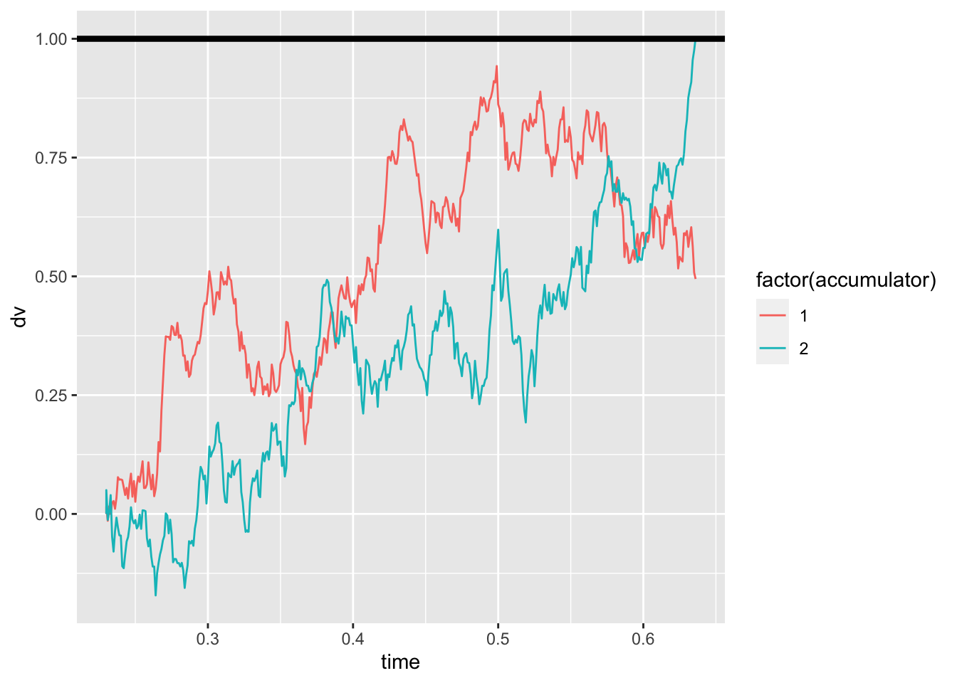
To have a look at the whole distribution, though, we want to simulate more trials:
random_rdm <- function(n_trials, drift1, drift2, threshold, ndt, sp1=0, sp2=0, noise_constant=1, dt=0.001, max_rt=10) {

  choice <- rep(NA, n_trials)
  rt <- rep(NA, n_trials)
  max_tsteps <- max_rt/dt

  # initialize the diffusion process
  tstep <- 0
  x1 <- rep(sp1*threshold, n_trials) # vector of accumulated evidence at t=tstep
  x2 <- rep(sp2*threshold, n_trials) # vector of accumulated evidence at t=tstep
  ongoing <- rep(TRUE, n_trials) # have the accumulators reached the bound?

  # start accumulating
  while (sum(ongoing) > 0 & tstep < max_tsteps) {
    x1[ongoing] <- x1[ongoing] + rnorm(mean=drift1*dt, sd=noise_constant*sqrt(dt), n=sum(ongoing))
    x2[ongoing] <- x2[ongoing] + rnorm(mean=drift2*dt, sd=noise_constant*sqrt(dt), n=sum(ongoing))
    tstep <- tstep + 1

    # ended trials
    ended1 <- (x1 >= threshold)
    ended2 <- (x2 >= threshold)

    # store results and filter out ended trials
    if(sum(ended1) > 0) {
      choice[ended1 & ongoing] <- 1
      rt[ended1 & ongoing] <- dt*tstep + ndt
      ongoing[ended1] <- FALSE
    }

    if(sum(ended2) > 0) {
      choice[ended2 & ongoing] <- 2
      rt[ended2 & ongoing] <- dt*tstep + ndt
      ongoing[ended2] <- FALSE
    }
  }
  return (data.frame(trial=seq(1, n_trials), choice=choice, rt=rt))
}
And have a look at the average performance and shape of the RT distributions:
sim_data <- random_rdm(n_trials=1000, drift1=.7, drift2=1.2, threshold=1.5, ndt=.23)
summary(sim_data)
## trial choice rt
## Min. : 1.0 Min. :1.000 Min. :0.3150
## 1st Qu.: 250.8 1st Qu.:1.000 1st Qu.:0.7518
## Median : 500.5 Median :2.000 Median :1.0115
## Mean : 500.5 Mean :1.643 Mean :1.1430
## 3rd Qu.: 750.2 3rd Qu.:2.000 3rd Qu.:1.3980
## Max. :1000.0 Max. :2.000 Max. :4.7470ggplot(data = sim_data, mapping = aes(x = rt, fill = factor(choice))) +
geom_histogram(binwidth=.05, alpha = .3, position="identity")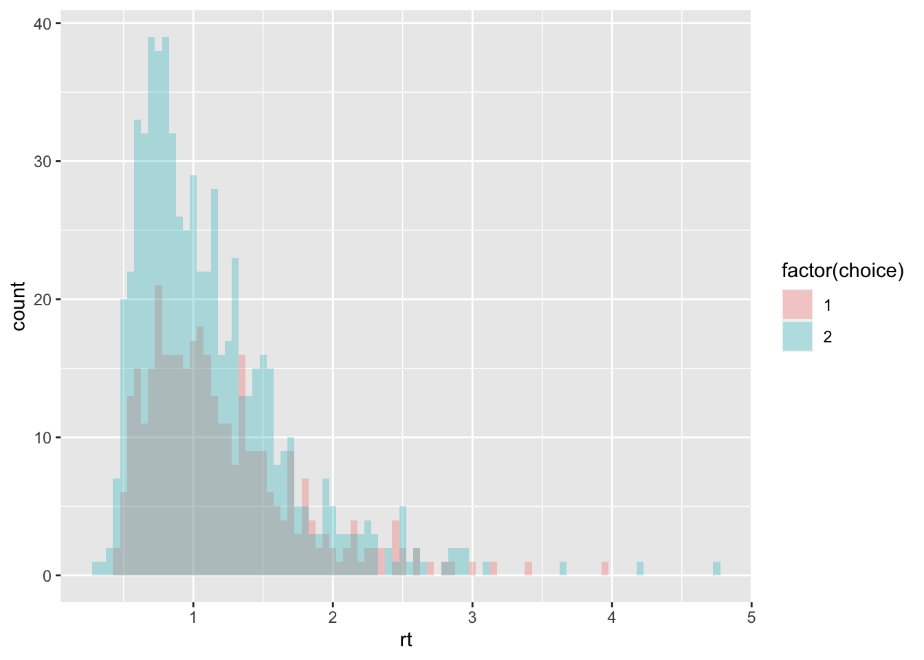
The same results can be obtained with the R code attached to the original paper, which can be downloaded and loaded in R:
sim_data <- rWaldRace(n=1000, v=c(.7, 1.2), B=1.5, A=0, t0=.23, gf = 0)
summary(sim_data)
## RT R
## Min. :0.3985 Min. :1.00
## 1st Qu.:0.7441 1st Qu.:1.00
## Median :0.9866 Median :2.00
## Mean :1.1444 Mean :1.64
## 3rd Qu.:1.3671 3rd Qu.:2.00
## Max. :4.8739 Max. :2.00Parameter recovery with MLE
In the same file, we can also find the likelihood function.
log_likelihood_rdm <- function(par, data, ll_threshold=1e-10) {
  # par order: drift1, drift2, threshold, ndt
  density <- rep(NA, dim(data)[1])
  data$RT <- (data$RT - par[4]) # shift the distribution by the NDT
  # dWald: density for single accumulator
  # pWald: cumulative density for single accumulator
  density[data$R==1] <- dWald(data$RT[data$R==1], v=par[1], B=par[3], A=0)*(1 - pWald(data$RT[data$R==1], v=par[2], B=par[3], A=0))
  density[data$R==2] <- dWald(data$RT[data$R==2], v=par[2], B=par[3], A=0)*(1 - pWald(data$RT[data$R==2], v=par[1], B=par[3], A=0))

  density[density <= ll_threshold] = ll_threshold # put a threhsold on very low likelihoods for computability

  return(sum(log(density)))
}

starting_values = c(1, 1, 1, .1) # set some starting values

print(log_likelihood_rdm(starting_values, data=sim_data))
## [1] -2033.958fit1 <- nmkb(par = starting_values,
fn = function (x) log_likelihood_rdm(x, data=sim_data),
lower = c(0, 0, 0, 0),
upper = c(10, 10, 10, 5),
control = list(maximize = TRUE))
print(fit1$par) # print estimated parameters## [1] 0.6788203 1.1721012 1.4287021 0.2572723Parameter Recovery with stan
We can also recover the generating parameters of the simulated data with stan, to assess th model’s identifialbility.
First, we need to prepare our data for stan:
sim_data_for_stan = list(
  N = dim(sim_data)[1],
  choices = sim_data$R,
  rt = sim_data$RT
)
And then we can fit the model:
fit1 <- stan(
  file = "stan_models/RDM.stan",                                 # Stan program
  data = sim_data_for_stan,                          # named list of data
  chains = 2,                                        # number of Markov chains
  warmup = 1000,                                     # number of warmup iterations per chain
  iter = 3000,                                       # total number of iterations per chain
  cores = 2                                          # number of cores (could use one per chain)
)
Compare the generating parameters with the recovered ones and check for convergence looking at the Rhat measures:
print(fit1, pars = c("transf_drift1", "transf_drift2", "transf_threshold", "transf_ndt"))## Inference for Stan model: RDM.
## 2 chains, each with iter=3000; warmup=1000; thin=1;
## post-warmup draws per chain=2000, total post-warmup draws=4000.
##
## mean se_mean sd 2.5% 25% 50% 75% 97.5% n_eff Rhat
## transf_drift1 0.68 0 0.07 0.55 0.64 0.68 0.73 0.81 1133 1
## transf_drift2 1.17 0 0.06 1.05 1.13 1.17 1.22 1.29 1010 1
## transf_threshold 1.44 0 0.07 1.31 1.39 1.43 1.48 1.58 924 1
## transf_ndt 0.25 0 0.02 0.21 0.24 0.25 0.27 0.29 1040 1
##
## Samples were drawn using NUTS(diag_e) at Wed Sep 8 23:24:18 2021.
## For each parameter, n_eff is a crude measure of effective sample size,
## and Rhat is the potential scale reduction factor on split chains (at
## convergence, Rhat=1).And (visually) assess the model’s convergence as well as some more sampling diagnostics:
traceplot(fit1, pars = c("transf_drift1", "transf_drift2", "transf_threshold", "transf_ndt"), inc_warmup = FALSE, nrow = 2)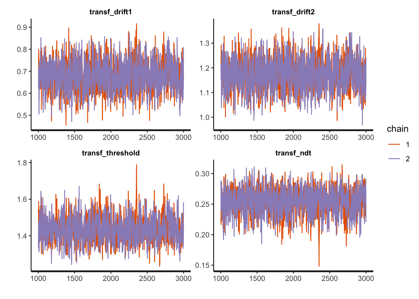
sampler_params <- get_sampler_params(fit1, inc_warmup = TRUE)
summary(do.call(rbind, sampler_params), digits = 2)
## accept_stat__ stepsize__ treedepth__ n_leapfrog__ divergent__ energy__
## Min. :0.00 Min. : 0.0028 Min. :0.0 Min. : 1 Min. :0.0000 Min. :1255
## 1st Qu.:0.88 1st Qu.: 0.2186 1st Qu.:3.0 1st Qu.: 7 1st Qu.:0.0000 1st Qu.:1257
## Median :0.96 Median : 0.2438 Median :3.0 Median : 15 Median :0.0000 Median :1258
## Mean :0.89 Mean : 0.2587 Mean :3.2 Mean : 14 Mean :0.0073 Mean :1260
## 3rd Qu.:0.99 3rd Qu.: 0.2438 3rd Qu.:4.0 3rd Qu.: 15 3rd Qu.:0.0000 3rd Qu.:1260
## Max. :1.00 Max. :14.3855 Max. :6.0 Max. :127 Max. :1.0000 Max. :2823More plotting:
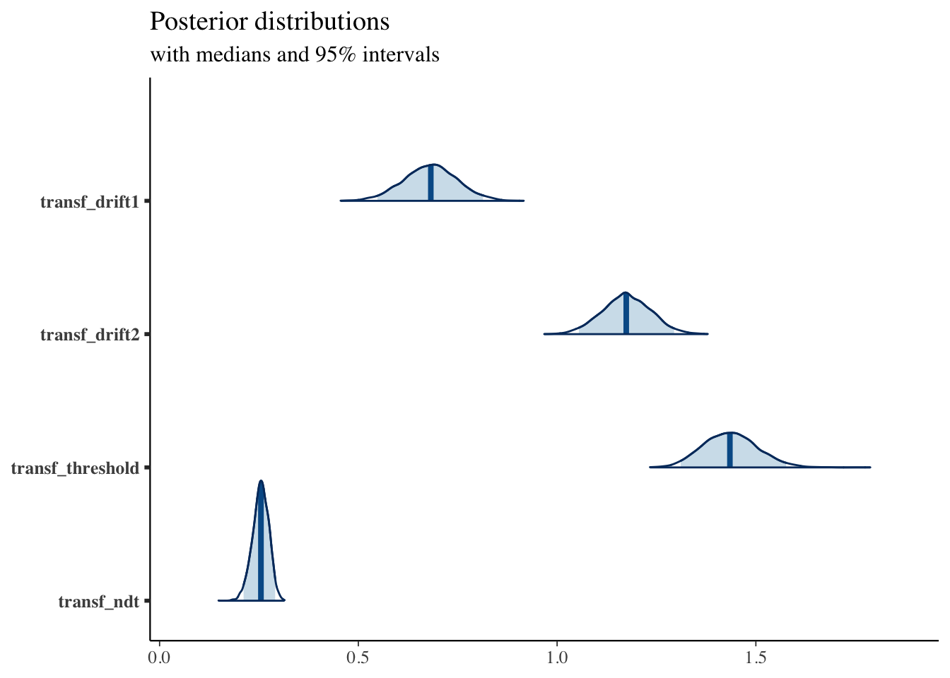
posterior <- as.matrix(fit1)

plot_title <- ggtitle("Posterior distributions",
                      "with medians and 95% intervals")
mcmc_areas(posterior,
           pars = c("transf_drift1", "transf_drift2", "transf_threshold", "transf_ndt"),
           prob = 0.95) + plot_title