The diffusion model
rm(list = ls())
library(tidyverse)
library(dfoptim)
library(rtdists)
library(rstan)
library(bayesplot)
We can write down Equation 5 from Bogacz 2006 paper to simulate the process described by the Diffusion Model without across-trial variability:
dm_path <- function(drift, threshold, ndt, rel_sp=.5, noise_constant=1, dt=0.001, max_rt=10) {
  max_tsteps <- max_rt/dt

  # initialize the diffusion process
  tstep <- 0
  x <- c(rel_sp*threshold) # vector of accumulated evidence at t=tstep
  time <- c(ndt)

  # start accumulating
  while (0 < x[tstep+1] & x[tstep+1] < threshold & tstep < max_tsteps) {
    x <- c(x, x[tstep+1] + rnorm(mean=drift*dt, sd=noise_constant*sqrt(dt), n=1))
    time <- c(time, dt*tstep + ndt)
    tstep <- tstep + 1
  }
  return (data.frame(time=time, dv=x))
}
And visualize it:
gen_drift = .3
gen_threshold = 1
gen_ndt = .23
sim_path <- dm_path(gen_drift, gen_threshold, gen_ndt)

ggplot(data = sim_path, aes(x = time, y = dv))+
  geom_line(size = .5) +
  geom_hline(yintercept=gen_threshold, size=1.5) +
  geom_hline(yintercept=0, size=1.5)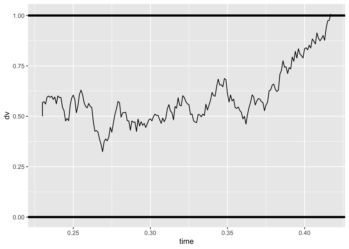
To have a look at the whole distribution, though, we want to simulate more trials:
random_dm <- function(n_trials, drift, threshold, ndt, rel_sp=.5, noise_constant=1, dt=0.001, max_rt=10) {

  acc <- rep(NA, n_trials)
  rt <- rep(NA, n_trials)
  max_tsteps <- max_rt/dt

  # initialize the diffusion process
  tstep <- 0
  x <- rep(rel_sp*threshold, n_trials) # vector of accumulated evidence at t=tstep
  ongoing <- rep(TRUE, n_trials) # have the accumulators reached the bound?

  # start accumulating
  while (sum(ongoing) > 0 & tstep < max_tsteps) {
    x[ongoing] <- x[ongoing] + rnorm(mean=drift*dt,
                                     sd=noise_constant*sqrt(dt),
                                     n=sum(ongoing))
    tstep <- tstep + 1

    # ended trials
    ended_correct <- (x >= threshold)
    ended_incorrect <- (x <= 0)

    # store results and filter out ended trials
    if(sum(ended_correct) > 0) {
      acc[ended_correct & ongoing] <- 1
      rt[ended_correct & ongoing] <- dt*tstep + ndt
      ongoing[ended_correct] <- FALSE
    }

    if(sum(ended_incorrect) > 0) {
      acc[ended_incorrect & ongoing] <- 0
      rt[ended_incorrect & ongoing] <- dt*tstep + ndt
      ongoing[ended_incorrect] <- FALSE
    }
  }
  return (data.frame(trial=seq(1, n_trials), accuracy=acc, rt=rt))
}
And have a look at the average performance and shape of the RT distributions:
sim_data <- random_dm(n_trials=1000, drift=.7, threshold=1.5, ndt=.23)
summary(sim_data)
## trial accuracy rt
## Min. : 1.0 Min. :0.000 Min. :0.2810
## 1st Qu.: 250.8 1st Qu.:1.000 1st Qu.:0.4657
## Median : 500.5 Median :1.000 Median :0.6575
## Mean : 500.5 Mean :0.752 Mean :0.7694
## 3rd Qu.: 750.2 3rd Qu.:1.000 3rd Qu.:0.9300
## Max. :1000.0 Max. :1.000 Max. :3.2900ggplot(data = sim_data, mapping = aes(x = rt, fill = factor(accuracy))) +
geom_histogram(binwidth=.05, alpha = .3, position="identity")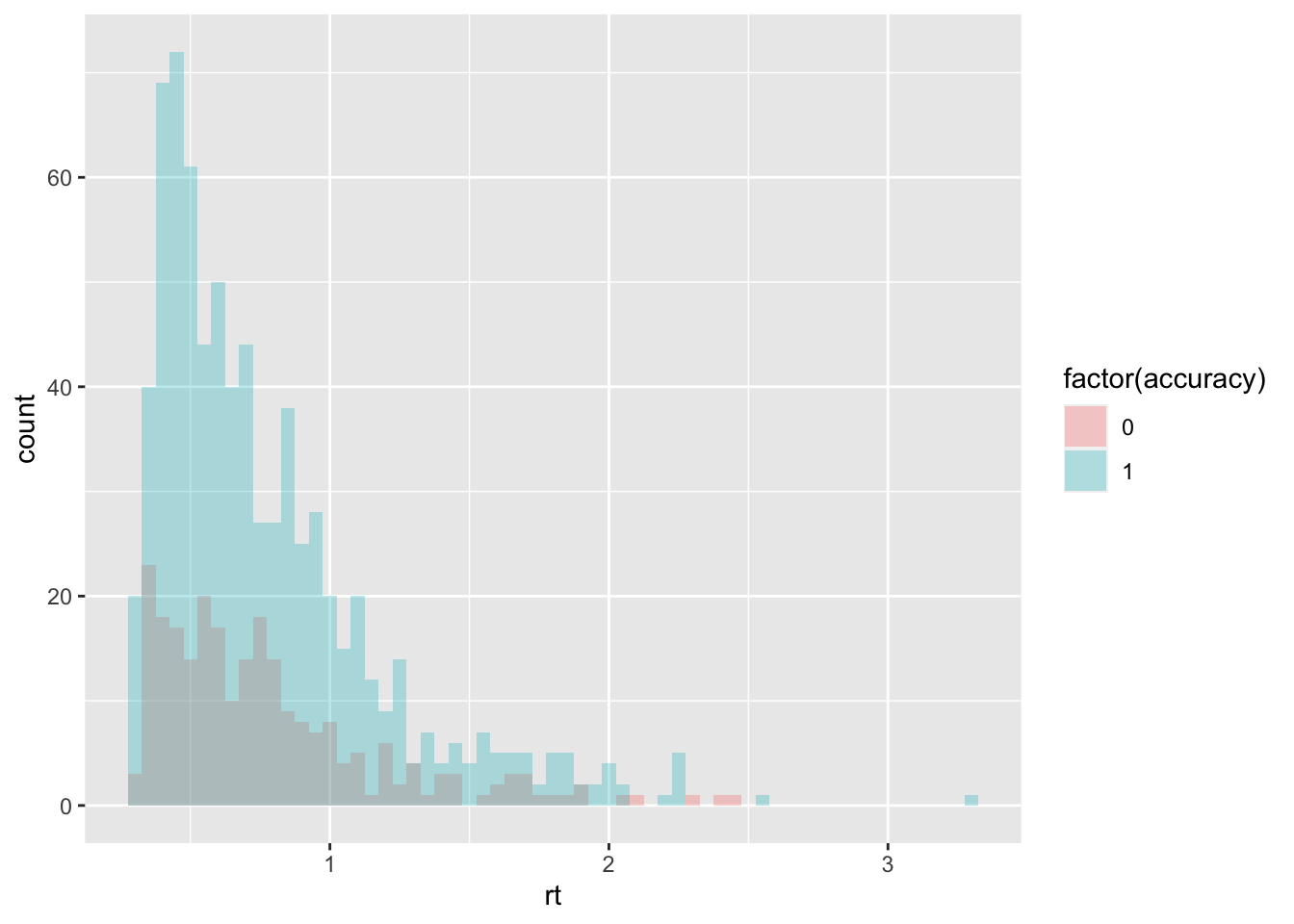
The same result can be achieved with the rdiffusion function of the rtdistspackage:
sim_data2 <- rdiffusion(n=1000, a=1.5, v=.7, t0=.23)
sim_data2$accuracy = 0
sim_data2[sim_data2$response=="upper", "accuracy"] = 1
summary(sim_data2)
## rt response accuracy
## Min. :0.2780 lower:242 Min. :0.000
## 1st Qu.:0.4545 upper:758 1st Qu.:1.000
## Median :0.6225 Median :1.000
## Mean :0.7387 Mean :0.758
## 3rd Qu.:0.8917 3rd Qu.:1.000
## Max. :2.6250 Max. :1.000Parameter recovery with MLE
An efficient approximation to the likelihood function of the DM can be found in the Navarro & Fuss paper. In the appendix, you can find the matlab code and convert it to R. However, a computationally efficient version of it can be also found in the rtdists package as well. We just need to wrap it to use in the MLE fitting later on:
log_likelihood_dm <- function(par, data, ll_threshold=1e-10) {

  density <- ddiffusion(rt=data$rt, response=data$response, a=par[1], v=par[2], t0=par[3])

  density[density <= ll_threshold] = ll_threshold # put a threhsold on very low likelihoods for computability

  return(sum(log(density)))
}
We can thus use the Nelder-Mead algorithm in the dfoptim package to estimate the parameters:
starting_values = c(.5, 1, .1) # set some starting values

print(log_likelihood_dm(starting_values, data=sim_data2)) # check that starting values are plausible
## [1] -9657.027fit1 <- nmkb(par = starting_values,
fn = function (x) log_likelihood_dm(x, data=sim_data2),
lower = c(0, -10, 0),
upper = c(10, 10, 5),
control = list(maximize = TRUE))
print(fit1$par) # print estimated parameters## [1] 1.4962874 0.7619161 0.2319887Parameter Recovery with stan
We can also recover the generating parameters of the simulated data with stan, to assess th model’s identifialbility.
First, we need to prepare our data for stan:
sim_data$accuracy_recoded = sim_data$accuracy
sim_data[sim_data$accuracy==0, "accuracy_recoded"] = -1

sim_data_for_stan = list(
  N = dim(sim_data)[1],
  accuracy = sim_data$accuracy_recoded,
  rt = sim_data$rt,
  starting_point = 0.5
)
And then we can fit the model:
fit1 <- stan(
  file = "stan_models/DM.stan",                      # Stan program
  data = sim_data_for_stan,                          # named list of data
  chains = 2,                                        # number of Markov chains
  warmup = 1000,                                     # number of warmup iterations per chain
  iter = 3000,                                       # total number of iterations per chain
  cores = 2                                          # number of cores (could use one per chain)
)
## Running /Library/Frameworks/R.framework/Resources/bin/R CMD SHLIB foo.c
## clang -mmacosx-version-min=10.13 -I"/Library/Frameworks/R.framework/Resources/include" -DNDEBUG -I"/Library/Frameworks/R.framework/Versions/4.0/Resources/library/Rcpp/include/" -I"/Library/Frameworks/R.framework/Versions/4.0/Resources/library/RcppEigen/include/" -I"/Library/Frameworks/R.framework/Versions/4.0/Resources/library/RcppEigen/include/unsupported" -I"/Library/Frameworks/R.framework/Versions/4.0/Resources/library/BH/include" -I"/Library/Frameworks/R.framework/Versions/4.0/Resources/library/StanHeaders/include/src/" -I"/Library/Frameworks/R.framework/Versions/4.0/Resources/library/StanHeaders/include/" -I"/Library/Frameworks/R.framework/Versions/4.0/Resources/library/RcppParallel/include/" -I"/Library/Frameworks/R.framework/Versions/4.0/Resources/library/rstan/include" -DEIGEN_NO_DEBUG -DBOOST_DISABLE_ASSERTS -DBOOST_PENDING_INTEGER_LOG2_HPP -DSTAN_THREADS -DBOOST_NO_AUTO_PTR -include '/Library/Frameworks/R.framework/Versions/4.0/Resources/library/StanHeaders/include/stan/math/prim/mat/fun/Eigen.hpp' -D_REENTRANT -DRCPP_PARALLEL_USE_TBB=1 -I/usr/local/include -fPIC -Wall -g -O2 -c foo.c -o foo.o
## In file included from <built-in>:1:
## In file included from /Library/Frameworks/R.framework/Versions/4.0/Resources/library/StanHeaders/include/stan/math/prim/mat/fun/Eigen.hpp:13:
## In file included from /Library/Frameworks/R.framework/Versions/4.0/Resources/library/RcppEigen/include/Eigen/Dense:1:
## In file included from /Library/Frameworks/R.framework/Versions/4.0/Resources/library/RcppEigen/include/Eigen/Core:88:
## /Library/Frameworks/R.framework/Versions/4.0/Resources/library/RcppEigen/include/Eigen/src/Core/util/Macros.h:613:1: error: unknown type name 'namespace'
## namespace Eigen {
## ^
## /Library/Frameworks/R.framework/Versions/4.0/Resources/library/RcppEigen/include/Eigen/src/Core/util/Macros.h:613:16: error: expected ';' after top level declarator
## namespace Eigen {
## ^
## ;
## In file included from <built-in>:1:
## In file included from /Library/Frameworks/R.framework/Versions/4.0/Resources/library/StanHeaders/include/stan/math/prim/mat/fun/Eigen.hpp:13:
## In file included from /Library/Frameworks/R.framework/Versions/4.0/Resources/library/RcppEigen/include/Eigen/Dense:1:
## /Library/Frameworks/R.framework/Versions/4.0/Resources/library/RcppEigen/include/Eigen/Core:96:10: fatal error: 'complex' file not found
## #include <complex>
## ^~~~~~~~~
## 3 errors generated.
## make: *** [foo.o] Error 1Compare the generating parameters with the recovered ones and check for convergence looking at the Rhat measures:
print(fit1, pars = c("drift", "transf_threshold", "transf_ndt"))## Inference for Stan model: DM.
## 2 chains, each with iter=3000; warmup=1000; thin=1;
## post-warmup draws per chain=2000, total post-warmup draws=4000.
##
## mean se_mean sd 2.5% 25% 50% 75% 97.5% n_eff Rhat
## drift 0.72 0 0.05 0.63 0.69 0.72 0.75 0.81 2701 1
## transf_threshold 1.53 0 0.02 1.48 1.51 1.53 1.55 1.58 2571 1
## transf_ndt 0.24 0 0.00 0.23 0.23 0.24 0.24 0.25 2605 1
##
## Samples were drawn using NUTS(diag_e) at Thu Sep 9 09:12:44 2021.
## For each parameter, n_eff is a crude measure of effective sample size,
## and Rhat is the potential scale reduction factor on split chains (at
## convergence, Rhat=1).And (visually) assess the model’s convergence as well as some more sampling diagnostics:
traceplot(fit1, pars = c("drift", "transf_threshold", "transf_ndt"), inc_warmup = FALSE, nrow = 2)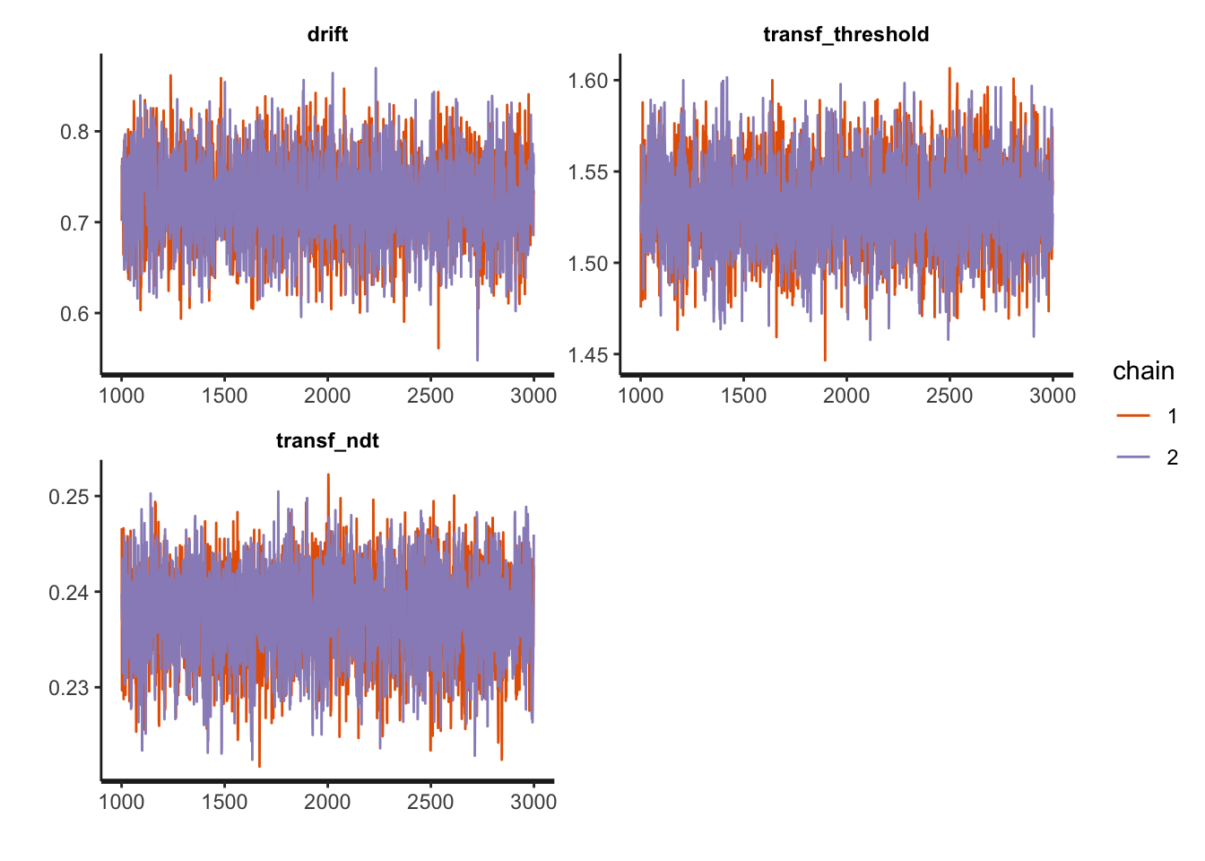
sampler_params <- get_sampler_params(fit1, inc_warmup = TRUE)
summary(do.call(rbind, sampler_params), digits = 2)
## accept_stat__ stepsize__ treedepth__ n_leapfrog__ divergent__
## Min. :0.00 Min. : 0.0023 Min. :0.0 Min. : 1.0 Min. :0.000
## 1st Qu.:0.85 1st Qu.: 0.6150 1st Qu.:2.0 1st Qu.: 3.0 1st Qu.:0.000
## Median :0.95 Median : 0.6265 Median :2.0 Median : 7.0 Median :0.000
## Mean :0.87 Mean : 0.6639 Mean :2.3 Mean : 5.6 Mean :0.005
## 3rd Qu.:0.99 3rd Qu.: 0.6265 3rd Qu.:3.0 3rd Qu.: 7.0 3rd Qu.:0.000
## Max. :1.00 Max. :14.4105 Max. :6.0 Max. :63.0 Max. :1.000
## energy__
## Min. : 791
## 1st Qu.: 793
## Median : 794
## Mean : 794
## 3rd Qu.: 795
## Max. :1205More plotting:
posterior <- as.matrix(fit1)

plot_title <- ggtitle("Posterior distributions",
                      "with medians and 95% intervals")
mcmc_areas(posterior,
           pars = c("drift", "transf_threshold", "transf_ndt"),
           prob = 0.95) + plot_title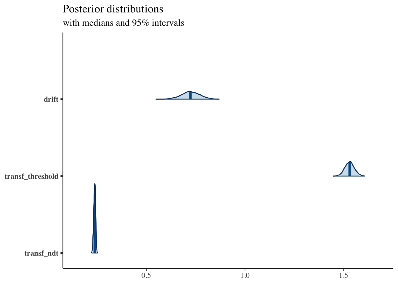
DM with across-trial variability in the drift-rate
Let’s now simulate data with across-trial variability in the drift-rate:
sim_data3 <- rdiffusion(n=1000, a=1.5, v=.7, t0=.23, sv=1)
sim_data3$accuracy = 0
sim_data3[sim_data3$response=="upper", "accuracy"] = 1
summary(sim_data3)
## rt response accuracy
## Min. :0.2585 lower:337 Min. :0.000
## 1st Qu.:0.4432 upper:663 1st Qu.:0.000
## Median :0.5952 Median :1.000
## Mean :0.7005 Mean :0.663
## 3rd Qu.:0.8179 3rd Qu.:1.000
## Max. :3.5134 Max. :1.000sim_data3$accuracy_recoded = sim_data3$accuracy
sim_data3[sim_data3$accuracy==0, "accuracy_recoded"] = -1
sim_data_for_stan = list(
N = dim(sim_data3)[1],
accuracy = sim_data3$accuracy_recoded,
rt = sim_data3$rt,
starting_point = 0.5
)And fit the model with across-trial variability in the drift-rate:
fit2 <- stan(
  file = "stan_models/DM_driftvar.stan",             # Stan program
  data = sim_data_for_stan,                          # named list of data
  chains = 2,                                        # number of Markov chains
  warmup = 1000,                                     # number of warmup iterations per chain
  iter = 3000,                                       # total number of iterations per chain
  cores = 2                                          # number of cores (could use one per chain)
)
## Running /Library/Frameworks/R.framework/Resources/bin/R CMD SHLIB foo.c
## clang -mmacosx-version-min=10.13 -I"/Library/Frameworks/R.framework/Resources/include" -DNDEBUG -I"/Library/Frameworks/R.framework/Versions/4.0/Resources/library/Rcpp/include/" -I"/Library/Frameworks/R.framework/Versions/4.0/Resources/library/RcppEigen/include/" -I"/Library/Frameworks/R.framework/Versions/4.0/Resources/library/RcppEigen/include/unsupported" -I"/Library/Frameworks/R.framework/Versions/4.0/Resources/library/BH/include" -I"/Library/Frameworks/R.framework/Versions/4.0/Resources/library/StanHeaders/include/src/" -I"/Library/Frameworks/R.framework/Versions/4.0/Resources/library/StanHeaders/include/" -I"/Library/Frameworks/R.framework/Versions/4.0/Resources/library/RcppParallel/include/" -I"/Library/Frameworks/R.framework/Versions/4.0/Resources/library/rstan/include" -DEIGEN_NO_DEBUG -DBOOST_DISABLE_ASSERTS -DBOOST_PENDING_INTEGER_LOG2_HPP -DSTAN_THREADS -DBOOST_NO_AUTO_PTR -include '/Library/Frameworks/R.framework/Versions/4.0/Resources/library/StanHeaders/include/stan/math/prim/mat/fun/Eigen.hpp' -D_REENTRANT -DRCPP_PARALLEL_USE_TBB=1 -I/usr/local/include -fPIC -Wall -g -O2 -c foo.c -o foo.o
## In file included from <built-in>:1:
## In file included from /Library/Frameworks/R.framework/Versions/4.0/Resources/library/StanHeaders/include/stan/math/prim/mat/fun/Eigen.hpp:13:
## In file included from /Library/Frameworks/R.framework/Versions/4.0/Resources/library/RcppEigen/include/Eigen/Dense:1:
## In file included from /Library/Frameworks/R.framework/Versions/4.0/Resources/library/RcppEigen/include/Eigen/Core:88:
## /Library/Frameworks/R.framework/Versions/4.0/Resources/library/RcppEigen/include/Eigen/src/Core/util/Macros.h:613:1: error: unknown type name 'namespace'
## namespace Eigen {
## ^
## /Library/Frameworks/R.framework/Versions/4.0/Resources/library/RcppEigen/include/Eigen/src/Core/util/Macros.h:613:16: error: expected ';' after top level declarator
## namespace Eigen {
## ^
## ;
## In file included from <built-in>:1:
## In file included from /Library/Frameworks/R.framework/Versions/4.0/Resources/library/StanHeaders/include/stan/math/prim/mat/fun/Eigen.hpp:13:
## In file included from /Library/Frameworks/R.framework/Versions/4.0/Resources/library/RcppEigen/include/Eigen/Dense:1:
## /Library/Frameworks/R.framework/Versions/4.0/Resources/library/RcppEigen/include/Eigen/Core:96:10: fatal error: 'complex' file not found
## #include <complex>
## ^~~~~~~~~
## 3 errors generated.
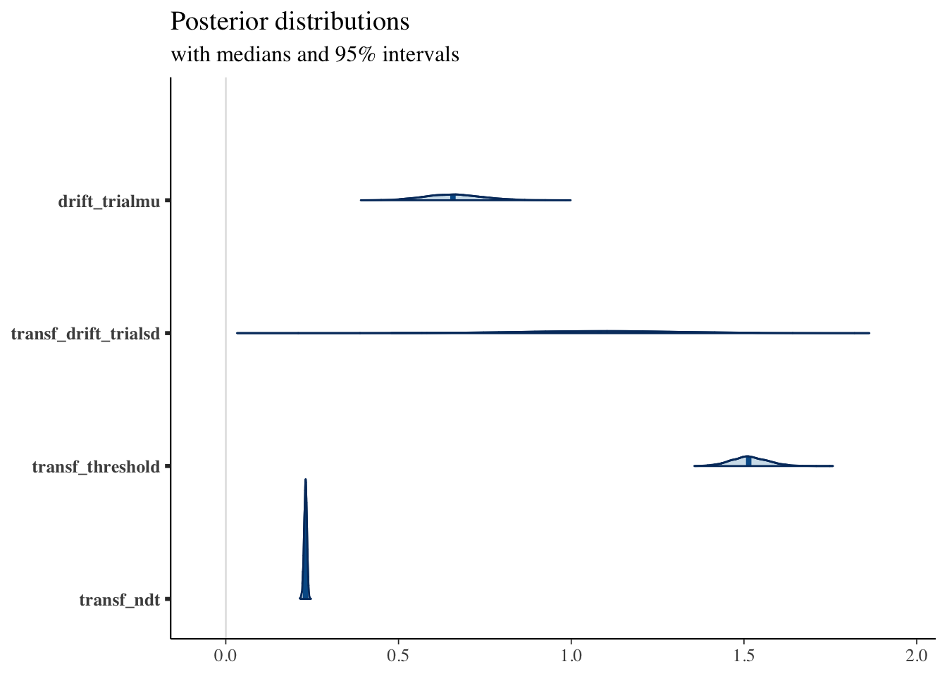
## make: *** [foo.o] Error 1Summary and plot:
print(fit2, pars = c("drift_trialmu", "transf_drift_trialsd", "transf_threshold", "transf_ndt"))## Inference for Stan model: DM_driftvar.
## 2 chains, each with iter=3000; warmup=1000; thin=1;
## post-warmup draws per chain=2000, total post-warmup draws=4000.
##
## mean se_mean sd 2.5% 25% 50% 75% 97.5% n_eff Rhat
## drift_trialmu 0.66 0.00 0.09 0.50 0.60 0.66 0.71 0.84 317 1
## transf_drift_trialsd 1.07 0.02 0.26 0.48 0.92 1.08 1.23 1.54 146 1
## transf_threshold 1.52 0.00 0.05 1.41 1.48 1.51 1.55 1.63 190 1
## transf_ndt 0.23 0.00 0.00 0.22 0.23 0.23 0.23 0.24 1027 1
##
## Samples were drawn using NUTS(diag_e) at Thu Sep 9 09:18:32 2021.
## For each parameter, n_eff is a crude measure of effective sample size,
## and Rhat is the potential scale reduction factor on split chains (at
## convergence, Rhat=1).posterior <- as.matrix(fit2)
plot_title <- ggtitle("Posterior distributions",
"with medians and 95% intervals")
mcmc_areas(posterior,
pars = c("drift_trialmu", "transf_drift_trialsd", "transf_threshold", "transf_ndt"),
prob = 0.95) + plot_title